For this case study, we will use the fairly well known Owl dataset which is provided in glmmTMB (see ?Owls for more info about the data). A frequentist base model would be:
library(glmmTMB)library(effects)
Loading required package: carData
lattice theme set by effectsTheme()
See ?effectsTheme for details.
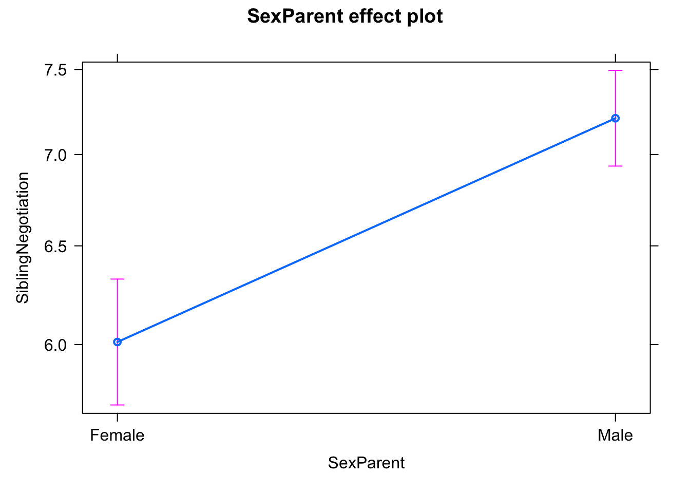
m1 <-glm(SiblingNegotiation ~ SexParent, data=Owls , family = poisson)summary(m1)
Call:
glm(formula = SiblingNegotiation ~ SexParent, family = poisson,
    data = Owls)

Deviance Residuals:
    Min       1Q   Median       3Q      Max
-3.7971  -3.4676  -0.4639   1.6272   6.7678

Coefficients:
              Estimate Std. Error z value Pr(>|z|)
(Intercept)    1.79380    0.02605  68.847  < 2e-16 ***
SexParentMale  0.18154    0.03272   5.548 2.89e-08 ***
---
Signif. codes:  0 '***' 0.001 '**' 0.01 '*' 0.05 '.' 0.1 ' ' 1

(Dispersion parameter for poisson family taken to be 1)

    Null deviance: 4290.9  on 598  degrees of freedom
Residual deviance: 4259.7  on 597  degrees of freedom
AIC: 5944.5

Number of Fisher Scoring iterations: 5
plot(allEffects(m1))
Exercise 1: fit this GLM using a Bayesian approach, e.g. Jags, STAN or brms
Tip
For STAN and JAGS, you will have to transform categorical variables to dummy coding, i.e.
sex =as.numeric(Owls$SexParent) -1
Then you can code
sexEffect * sex[i]
Exercise 2: include a log offset to the model too account for BroodSize
m2 <-glm(SiblingNegotiation ~ FoodTreatment*SexParent +offset(log(BroodSize)), data=Owls , family = poisson)
Exercise 3: check residuals and / or add obvious additional components to the model inspired by the frequentist example here.
This is DHARMa 0.4.6. For overview type '?DHARMa'. For recent changes, type news(package = 'DHARMa')
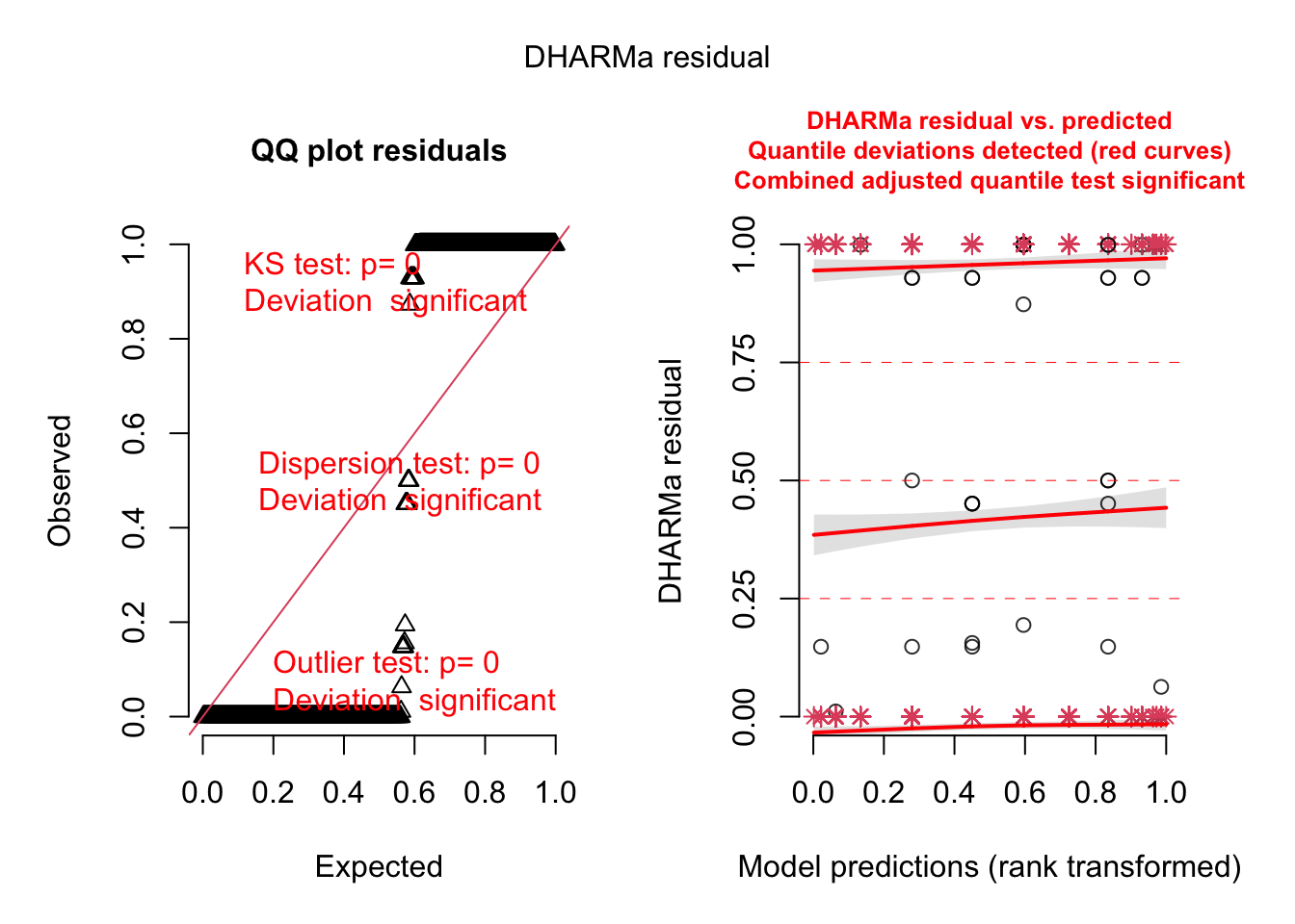
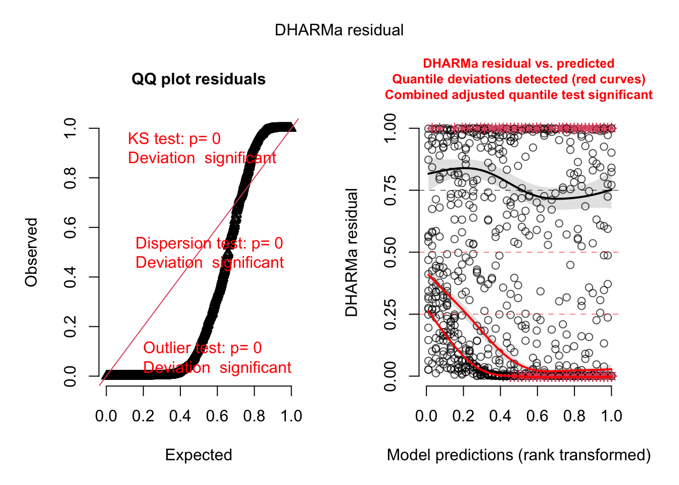
x =getSample(Samples)# note - yesterday, we calcualted the predictions from the parameters# here we observe them direct - this is the normal way to calcualte the # posterior predictive distributionposteriorPredDistr = x[,5:(4+599)]posteriorPredSim = x[,(5+599):(4+2*599)]sim =createDHARMa(simulatedResponse =t(posteriorPredSim), observedResponse = Owls$SiblingNegotiation, fittedPredictedResponse =apply(posteriorPredDistr, 2, median), integerResponse = T)plot(sim)
DHARMa:testOutliers with type = binomial may have inflated Type I error rates for integer-valued distributions. To get a more exact result, it is recommended to re-run testOutliers with type = 'bootstrap'. See ?testOutliers for details
Solution using brms
Here a base model with random effect
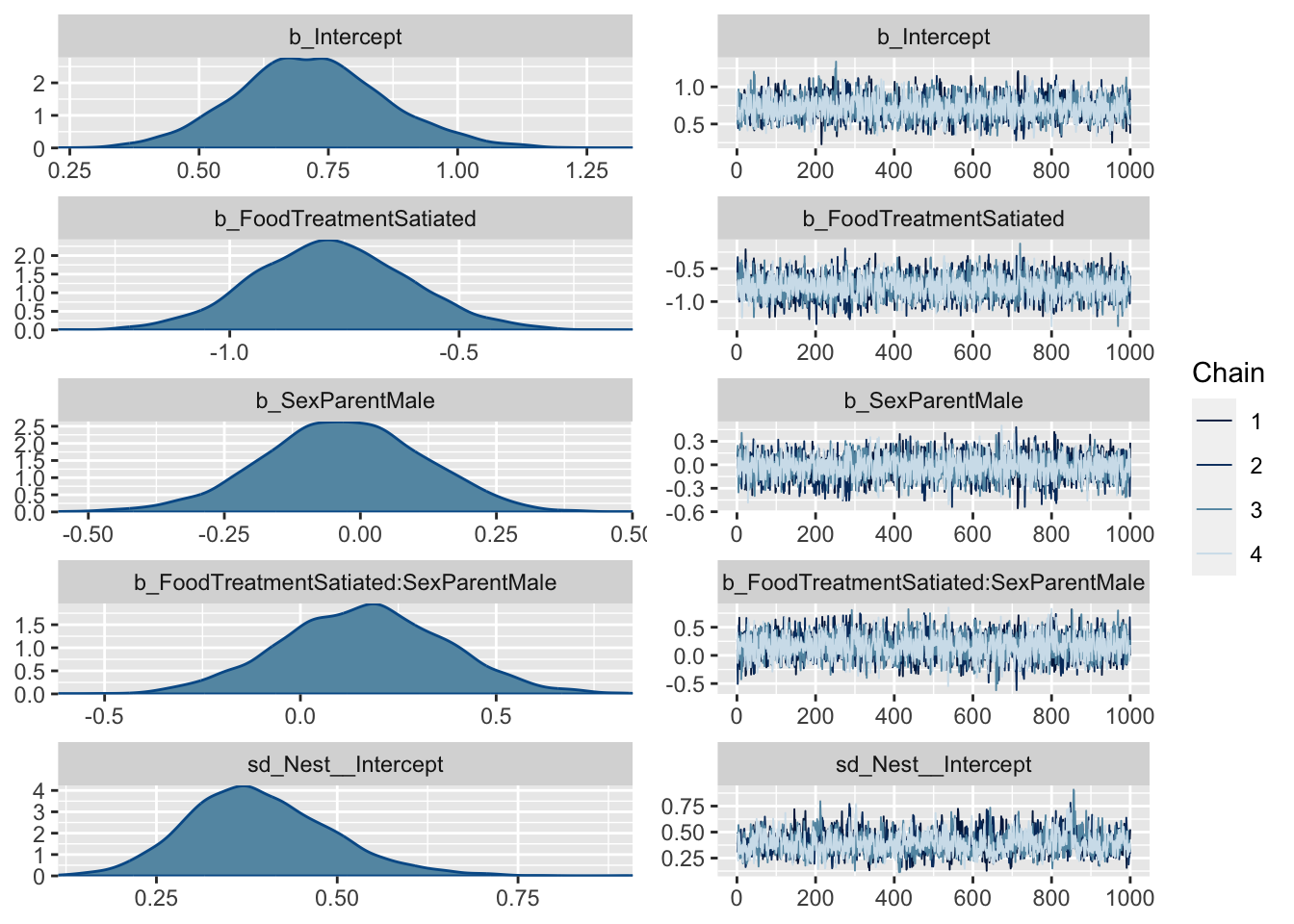
library(brms)m2 = brms::brm(SiblingNegotiation ~ FoodTreatment * SexParent+ (1|Nest) +offset(log(BroodSize)), data = Owls , family = negbinomial)
Family: negbinomial
Links: mu = log; shape = identity
Formula: SiblingNegotiation ~ FoodTreatment * SexParent + (1 | Nest) + offset(log(BroodSize))
Data: Owls (Number of observations: 599)
Draws: 4 chains, each with iter = 2000; warmup = 1000; thin = 1;
total post-warmup draws = 4000
Group-Level Effects:
~Nest (Number of levels: 27)
Estimate Est.Error l-95% CI u-95% CI Rhat Bulk_ESS Tail_ESS
sd(Intercept) 0.39 0.10 0.22 0.61 1.00 1034 1605
Population-Level Effects:
Estimate Est.Error l-95% CI u-95% CI Rhat
Intercept 0.72 0.14 0.44 1.02 1.00
FoodTreatmentSatiated -0.78 0.17 -1.11 -0.43 1.00
SexParentMale -0.03 0.15 -0.33 0.25 1.00
FoodTreatmentSatiated:SexParentMale 0.16 0.21 -0.25 0.57 1.00
Bulk_ESS Tail_ESS
Intercept 2621 2779
FoodTreatmentSatiated 3128 3210
SexParentMale 3373 2454
FoodTreatmentSatiated:SexParentMale 3079 3016
Family Specific Parameters:
Estimate Est.Error l-95% CI u-95% CI Rhat Bulk_ESS Tail_ESS
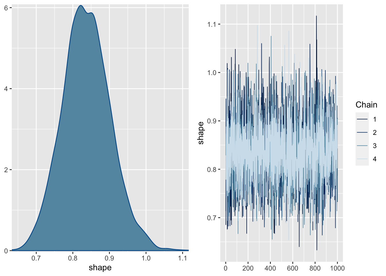
shape 0.84 0.07 0.71 0.97 1.00 5786 2933
Draws were sampled using sampling(NUTS). For each parameter, Bulk_ESS
and Tail_ESS are effective sample size measures, and Rhat is the potential
scale reduction factor on split chains (at convergence, Rhat = 1).
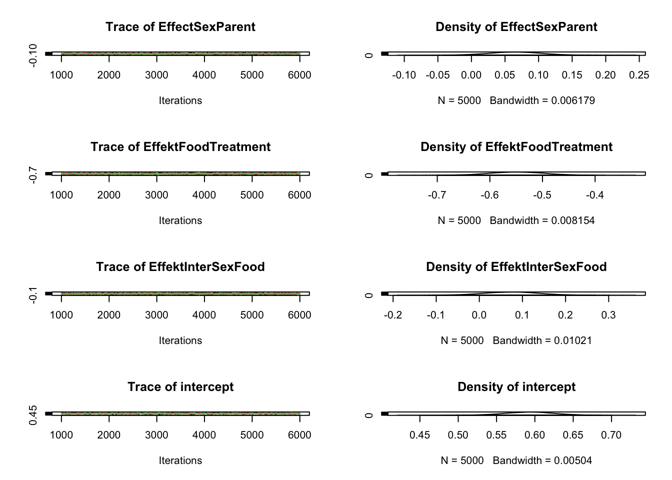
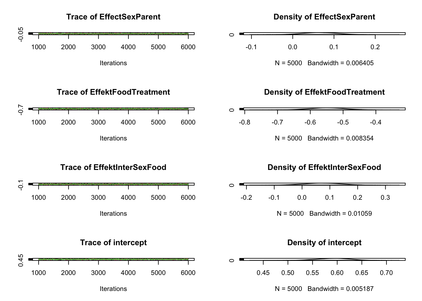
plot(m2, ask =FALSE)
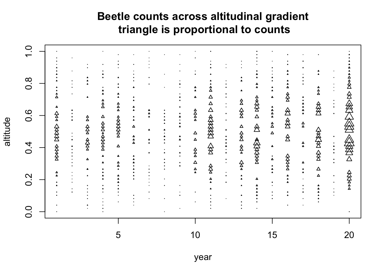
C.2 Beetles
# This first part creates a dataset with beetles counts across an altitudinal gradient (several plots each observed several years), with a random intercept on year and zero-inflation. altitude =rep(seq(0,1,len =50), each =20)dataID =1:1000spatialCoordinate =rep(seq(0,30, len =50), each =20)# random effects + zeroinflationplot =rep(1:50, each =20)year =rep(1:20, times =50)yearRandom =rnorm(20, 0, 1)plotRandom =rnorm(50, 0, 1)overdispersion =rnorm(1000, sd =0.5)zeroinflation =rbinom(1000,1,0.6)beetles <-rpois(1000, exp( 0+12*altitude -12*altitude^2# + overdispersion + plotRandom[plot]+ yearRandom[year]) * zeroinflation )data =data.frame(dataID, beetles, altitude, plot, year, spatialCoordinate)plot(year, altitude, cex = beetles/50, pch =2, main ="Beetle counts across altitudinal gradient\n triangle is proportional to counts")
library(R2jags)
Attaching package: 'R2jags'
The following object is masked from 'package:coda':

    traceplot
plotSimulatedResiduals is deprecated, please switch your code to simply using the plot() function
DHARMa:testOutliers with type = binomial may have inflated Type I error rates for integer-valued distributions. To get a more exact result, it is recommended to re-run testOutliers with type = 'bootstrap'. See ?testOutliers for details
qu = 0.25, log(sigma) = -4.086977 : outer Newton did not converge fully.
C.3 CNDD estimated, Comita et al., 2010
This is the model from Comita, L. S., Muller-Landau, H. C., Aguilar, S., & Hubbell, S. P. (2010). Asymmetric density dependence shapes species abundances in a tropical tree community. Science, 329(5989), 330-332.
The model was originally written in WinBugs. The version here was here slightly modified to be run with JAGS. Rerunning these models were part of the tests we did to settle on the methodology in Hülsmann, L., Chisholm, R. A., Comita, L., Visser, M. D., de Souza Leite, M., Aguilar, S., … & Hartig, F. (2024). Latitudinal patterns in stabilizing density dependence of forest communities. Nature, 1-8.
Our tests indicated that this model is excellent in recovering CNDD estimates from simulations. The main reason we didn’t use a similar model in Hülsmann et al., 2024 were computational limitations and the difficulty to include splines on the species-specific density responses in such a hierarchical setting.
Task: go through the paper and the code and try to understand what the structure of the model!
model{for (i in1:N) { SD[i] ~dbern(p[i]) SD_sim[i] ~dbern(p[i])logit(p[i]) <- B[SPP[i], ] %*% PREDS[i, ] + u[PLOT[i]] }# Standard Random intercept on plotfor (m in1:Nplots) { u[m] ~dnorm(0, a.tau) } a.sigma ~dunif(0, 100) a.tau <-1/ (a.sigma * a.sigma)#redundant parameterization speeds convergence in WinBugs, see Gelman & Hill (2007)for (k in1:K) {for (j in1:Nspp) { B[j, k] <- xi[k] * B.raw[j, k] } xi[k] ~dunif(0, 100) }#multivariate normal distribution for B values of each speciesfor (j in1:Nspp) { B.raw[j, 1:K] ~dmnorm(B.raw.hat[j, ], Tau.B.raw[, ])#G.raw is matrix of regression coefficients for species-level model#ABUND is species-level predictors (abundance and shade tolerance)for (k in1:K) { B.raw.hat[j, k] <- G.raw[k, ] %*% ABUND[j, ] # ABUND needs to be matrix w/ 1st column all 1's } }#priors for G and redundant parameterizationfor (k in1:K) {for (l in1:3) { G[k, l] <- xi[k] * G.raw[k, l] G.raw[k, l] ~dnorm(0, 0.1) } }#covariance matrix modeled using scaled inverse wishart model Tau.B.raw[1:K, 1:K] ~dwish(W[, ], df) df <- K +1 Sigma.B.raw[1:K, 1:K] <-inverse(Tau.B.raw[, ])# correlationsfor (k in1:K) {for (k.prime in1:K) { rho.B[k, k.prime] <- Sigma.B.raw[k, k.prime] /sqrt(Sigma.B.raw[k, k] * Sigma.B.raw[k.prime, k.prime]) }# sigma.B[k] <-abs(xi[k]) *sqrt(Sigma.B.raw[k, k]) }################ Predictions ############# Addition to original model (Nov 2019)# to estimate the effect of mortality (response) when changing 1 unit on x-axis# data (old, read with the name 'txt') is centered but not scaled, therefore 'zero' is here the value of '-6.81'for (i in1:N) { baseMort[i] =ilogit(B[SPP[i], 1] * PREDS[i, 1] + B[SPP[i], 2] * (-6.81) + B[SPP[i], 3:5] %*% PREDS[i, 3:5]) conMort[i] =ilogit(B[SPP[i], 1] * PREDS[i, 1] + B[SPP[i], 2] * (-5.81) + B[SPP[i], 3:5] %*% PREDS[i, 3:5])# relConEffekt[i] <- (conMort[i] - baseMort[i]) / baseMort[i]# hetEffekt[i] <- ilogit(B[SPP[i],1] * PREDS[i,1] + B[SPP[i],2] * PREDS[i,3]^CC[SPP[i]] + B[SPP[i],3] * 1 + B[SPP[i],4:5] %*% PREDS[i,4:5]) - ilogit(B[SPP[i],1] * PREDS[i,1] + B[SPP[i],2] * PREDS[i,3]^CC[SPP[i]] + B[SPP[i],3] * 0 + B[SPP[i],4:5] %*% PREDS[i,4:5]) }}
Call:
lm(formula = y ~ x)

Residuals:
   Min     1Q Median     3Q    Max
-47.21 -21.53  -4.41  11.95  71.57

Coefficients:
            Estimate Std. Error t value Pr(>|t|)
(Intercept)  25.6079     4.0436   6.333 5.32e-08 ***
x             4.5581     0.2547  17.894  < 2e-16 ***
---
Signif. codes:  0 '***' 0.001 '**' 0.01 '*' 0.05 '.' 0.1 ' ' 1

Residual standard error: 29.99 on 53 degrees of freedom
Multiple R-squared:  0.858, Adjusted R-squared:  0.8553
F-statistic: 320.2 on 1 and 53 DF,  p-value: < 2.2e-16
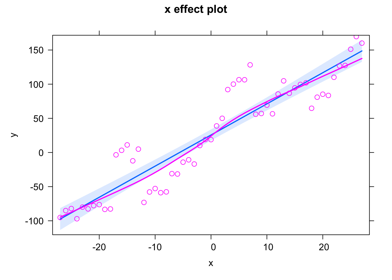
plot(allEffects(fit, partial.residuals = T))
## ---- fig.width=5, fig.height=5------------------------------------------fit <-lmer(y ~ x + (1|group))summary(fit)
Linear mixed model fit by REML ['lmerMod']
Formula: y ~ x + (1 | group)

REML criterion at convergence: 438.2

Scaled residuals:
     Min       1Q   Median       3Q      Max
-1.81013 -0.60007 -0.07453  0.70328  1.91655

Random effects:
 Groups   Name        Variance Std.Dev.
 group    (Intercept) 925.64   30.424
 Residual              89.63    9.467
Number of obs: 55, groups:  group, 11

Fixed effects:
            Estimate Std. Error t value
(Intercept)  25.6079     9.2617   2.765
x             4.6488     0.4914   9.461

Correlation of Fixed Effects:
  (Intr)
x 0.000
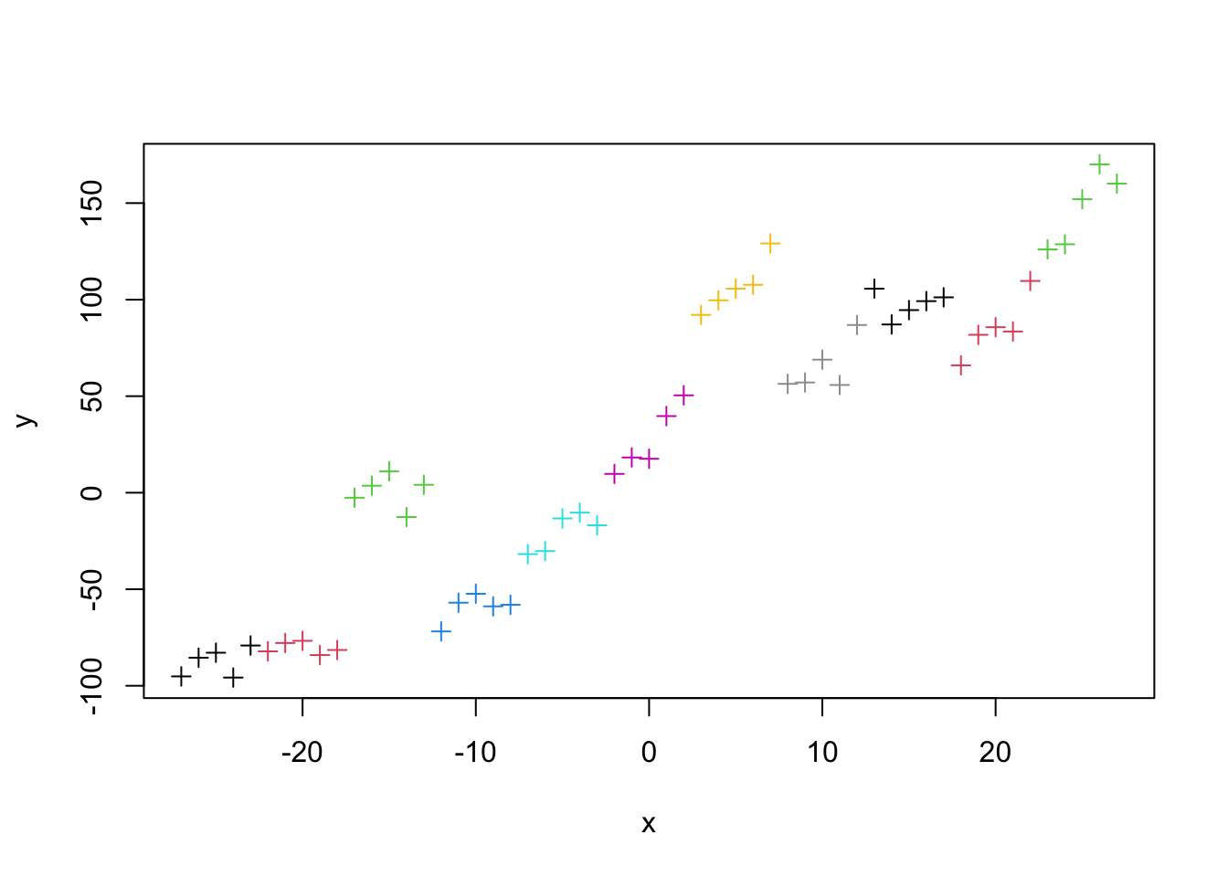
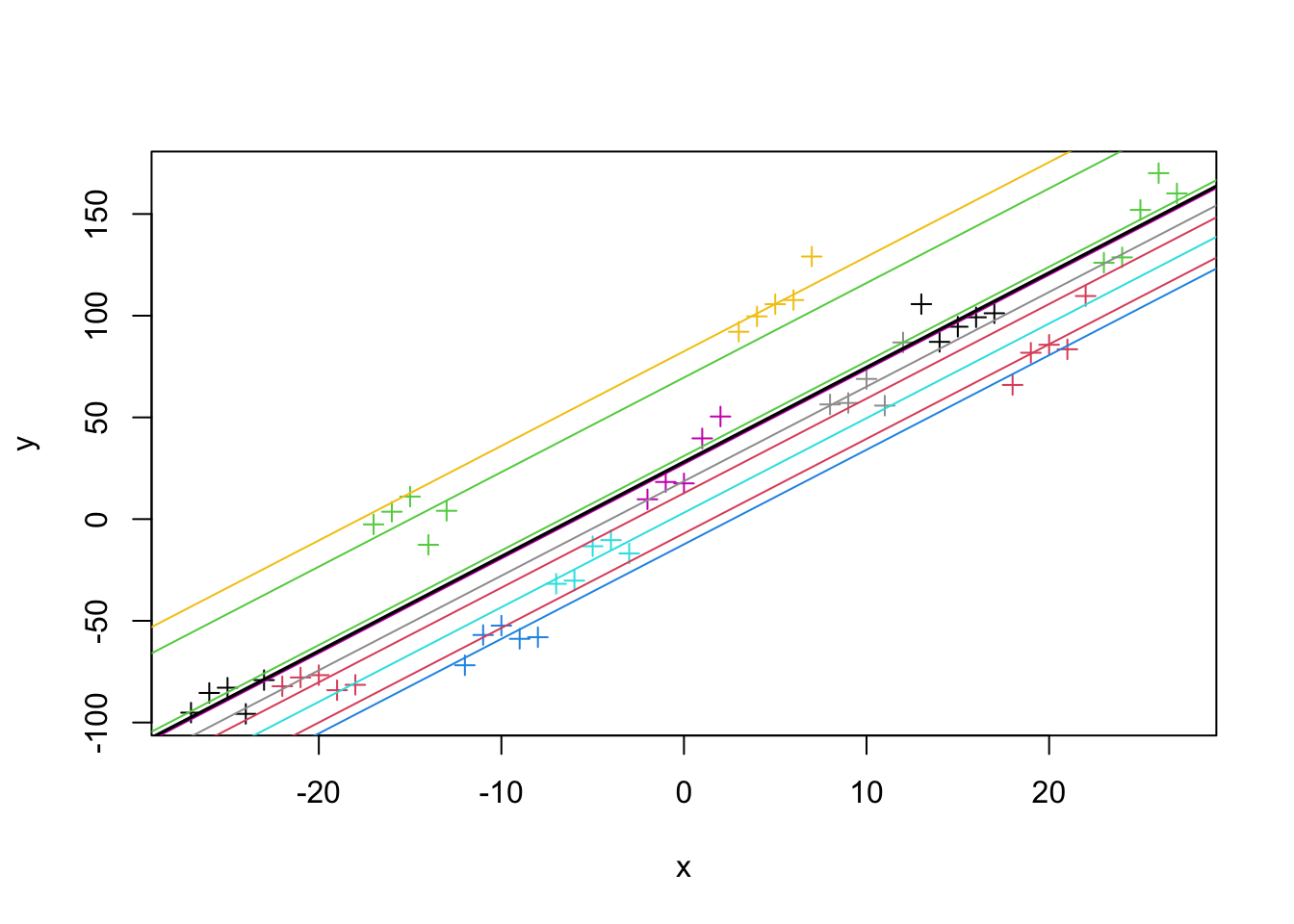
plot(x,y, col = group, pch =3)for(i in1:11){abline(coef(fit)$group[i,1], coef(fit)$group[i,2], col = i)}
## ------------------------------------------------------------------------# 1) Model definition exactly how we created our data modelCode =" model{ # Likelihood for(i in 1:i.max){ y[i] ~ dnorm(mu[i],tau) mu[i] <- a*x[i] + b } # Prior distributions a ~ dnorm(0,0.001) b ~ dnorm(0,0.001) tau <- 1/(sigma*sigma) sigma ~ dunif(0,100) } "# 2) Set up a list that contains all the necessary data (here, including parameters of the prior distribution) Data =list(y = y, x = x, i.max =length(y))# 3) Specify a function to generate inital values for the parameters inits.fn <-function() list(a =rnorm(1), b =rnorm(1), sigma =runif(1,1,100))## ---- fig.width=7, fig.height=7------------------------------------------# Compile the model and run the MCMC for an adaptation (burn-in) phase jagsModel <-jags.model(file=textConnection(modelCode), data=Data, init = inits.fn, n.chains =3, n.adapt=1000)
Compiling model graph
   Resolving undeclared variables
   Allocating nodes
Graph information:
   Observed stochastic nodes: 55
   Unobserved stochastic nodes: 3
   Total graph size: 230

Initializing model
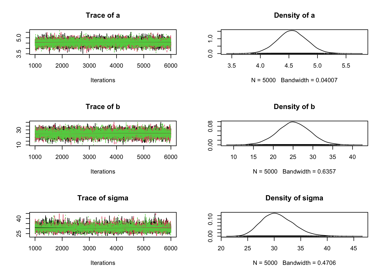
# Specify parameters for which posterior samples are saved para.names <-c("a","b","sigma")# Continue the MCMC runs with sampling Samples <-coda.samples(jagsModel, variable.names = para.names, n.iter =5000)# Plot the mcmc chain and the posterior sample for pplot(Samples)
dic =dic.samples(jagsModel, n.iter =5000) dic
Mean deviance:  531.3
penalty 3.12
Penalized deviance: 534.4
Iterations = 1001:6000
Thinning interval = 1
Number of chains = 3
Sample size per chain = 5000

1. Empirical mean and standard deviation for each variable,
   plus standard error of the mean:

        Mean    SD Naive SE Time-series SE
a      4.556 0.261 0.002131       0.002111
b     25.151 4.127 0.033694       0.033694
sigma 30.703 3.038 0.024803       0.033976

2. Quantiles for each variable:

        2.5%    25%    50%   75%  97.5%
a      4.044  4.383  4.554  4.73  5.069
b     16.946 22.427 25.159 27.93 33.239
sigma 25.443 28.538 30.458 32.64 37.230
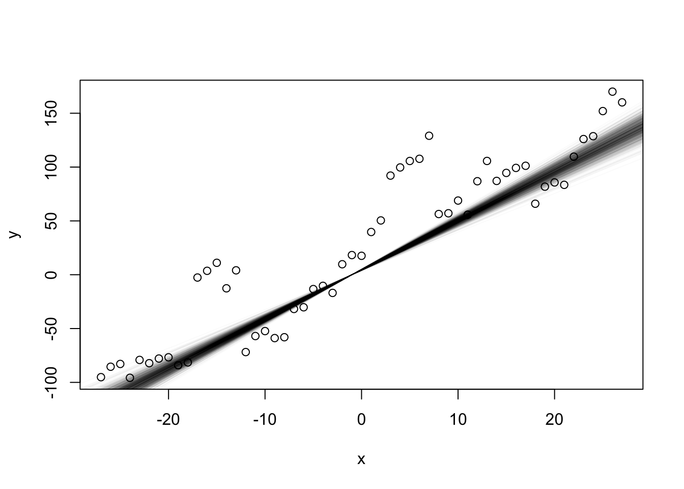
## ---- fig.width=5, fig.height=5------------------------------------------plot(x,y)sampleMatrix <-as.matrix(Samples)selection <-sample(dim(sampleMatrix)[1], 1000)for (i in selection) abline(sampleMatrix[i,1], sampleMatrix[i,1], col ="#11111105")
Alternative: mixed model
## ------------------------------------------------------------------------# 1) Model definition exactly how we created our data modelCode =" model{ # Likelihood for(i in 1:i.max){ y[i] ~ dnorm(mu[i],tau) mu[i] <- a*x[i] + b + r[group[i]] } # random effect for(i in 1:nGroups){ r[i] ~ dnorm(0,rTau) } # Prior distributions a ~ dnorm(0,0.001) b ~ dnorm(0,0.001) tau <- 1/(sigma*sigma) sigma ~ dunif(0,100) rTau <- 1/(rSigma*rSigma) rSigma ~ dunif(0,100) } "# 2) Set up a list that contains all the necessary data (here, including parameters of the prior distribution) Data =list(y = y, x = x, i.max =length(y), group = group, nGroups =11)# 3) Specify a function to generate inital values for the parameters inits.fn <-function() list(a =rnorm(1), b =rnorm(1), sigma =runif(1,1,100), rSigma =runif(1,1,100))## ---- fig.width=7, fig.height=7------------------------------------------# Compile the model and run the MCMC for an adaptation (burn-in) phase jagsModel <-jags.model(file=textConnection(modelCode), data=Data, init = inits.fn, n.chains =3, n.adapt=1000)
Compiling model graph
   Resolving undeclared variables
   Allocating nodes
Graph information:
   Observed stochastic nodes: 55
   Unobserved stochastic nodes: 15
   Total graph size: 300

Initializing model
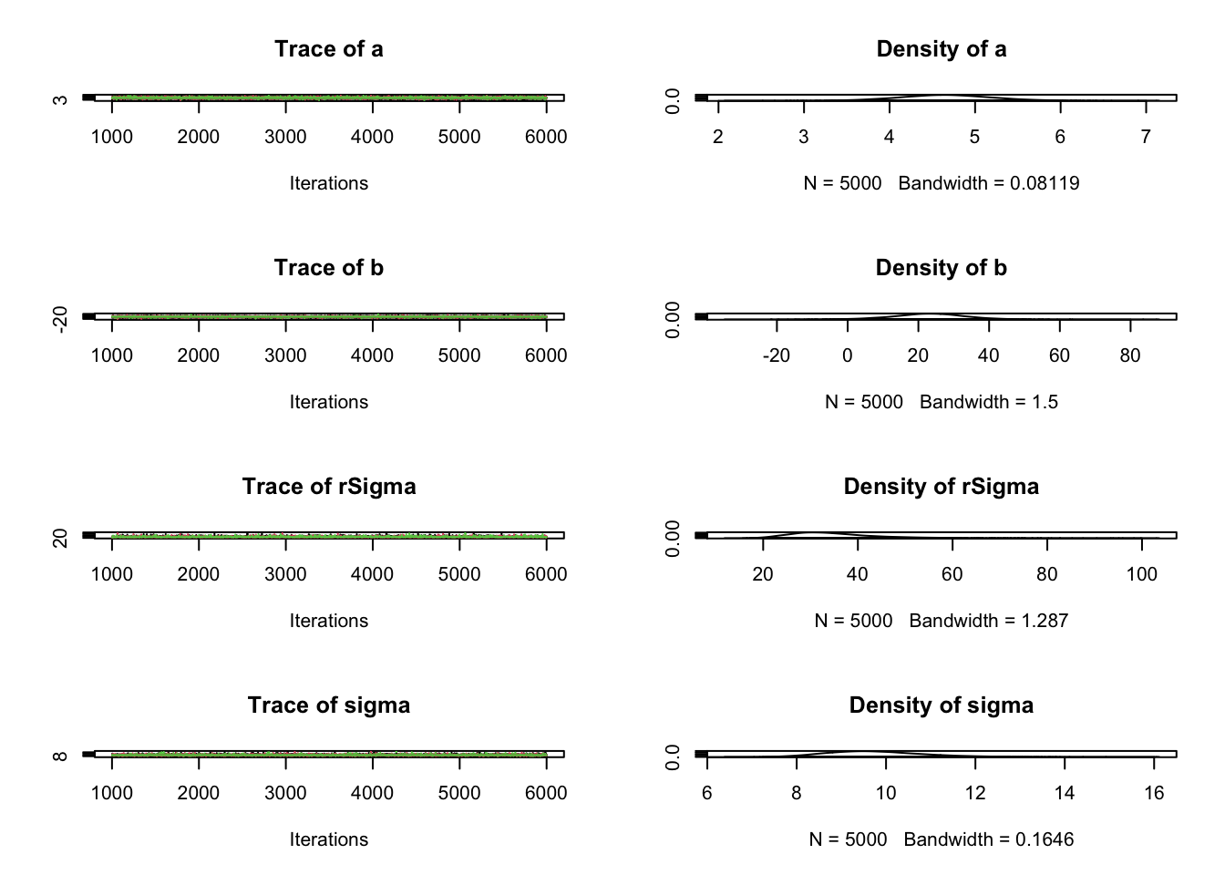
# Specify parameters for which posterior samples are saved para.names <-c("a","b","sigma", "rSigma")# Continue the MCMC runs with sampling Samples <-coda.samples(jagsModel, variable.names = para.names, n.iter =5000)# Plot the mcmc chain and the posterior sample for pplot(Samples)