Dat <- read.table('https://raw.githubusercontent.com/florianhartig/LearningBayes/master/data/LizardData.txt')
plot(Dat$Veg,Dat$Count)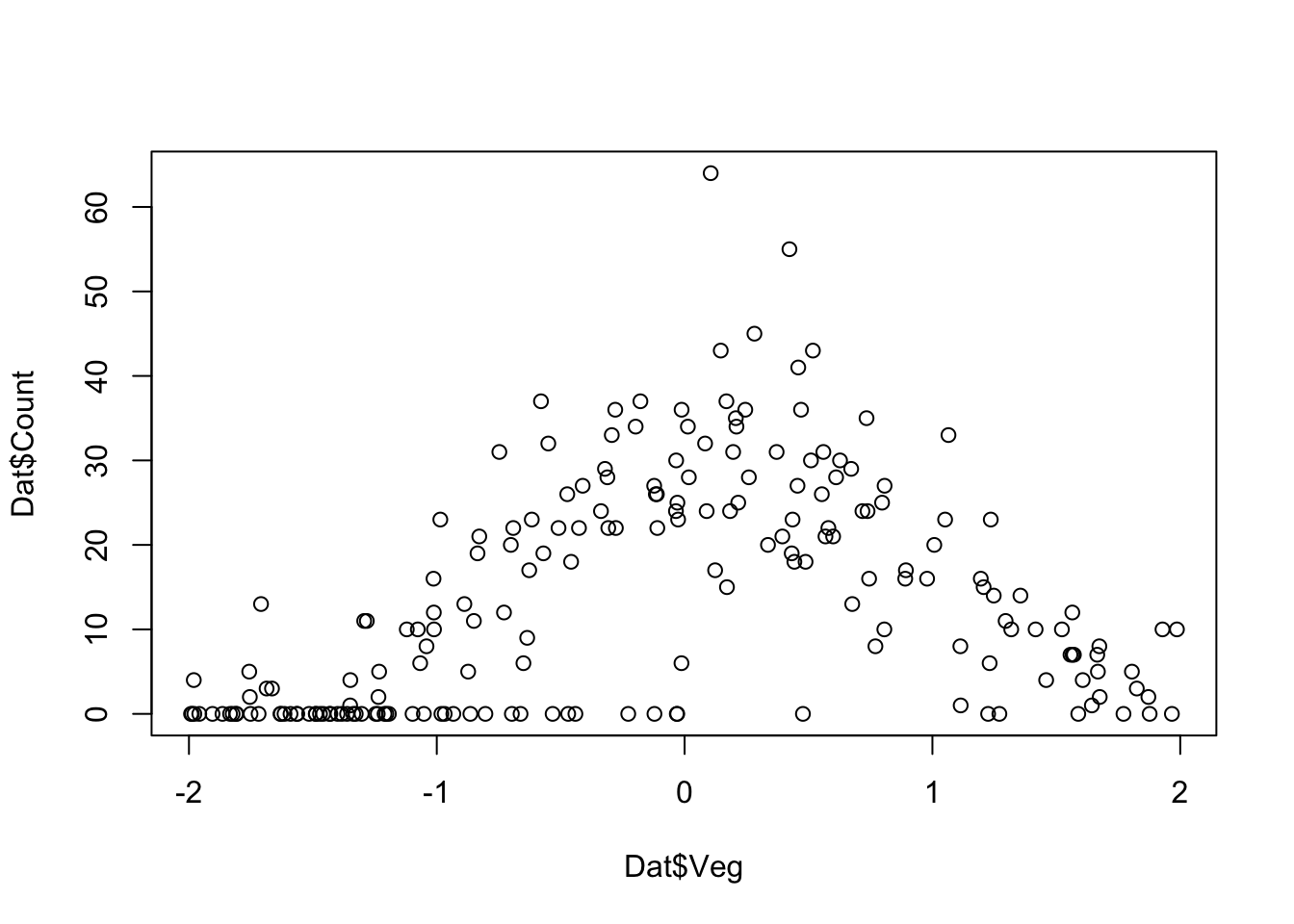
Dat <- read.table('https://raw.githubusercontent.com/florianhartig/LearningBayes/master/data/LizardData.txt')
plot(Dat$Veg,Dat$Count)
Standard frequentist GLM
fit <- glm(Count ~ Veg, data = Dat, family = "poisson")
summary(fit)
Call:
glm(formula = Count ~ Veg, family = "poisson", data = Dat)

Deviance Residuals:
    Min       1Q   Median       3Q      Max
-6.8004  -4.2794  -0.9161   2.4673   9.6535

Coefficients:
            Estimate Std. Error z value Pr(>|z|)
(Intercept)  2.62494    0.01923  136.50   <2e-16 ***
Veg          0.26236    0.01736   15.11   <2e-16 ***
---
Signif. codes:  0 '***' 0.001 '**' 0.01 '*' 0.05 '.' 0.1 ' ' 1

(Dispersion parameter for poisson family taken to be 1)

    Null deviance: 3015.9  on 199  degrees of freedom
Residual deviance: 2785.7  on 198  degrees of freedom
AIC: 3433.1

Number of Fisher Scoring iterations: 6library(rjags)
library(DHARMa)
library(BayesianTools)
# Model specification
model = "
model{
# Likelihood
for(i in 1:n.dat){
# poisson model p(y|lambda)
y[i] ~ dpois(lambda[i])
# logit link function
log(lambda[i]) <- mu[i]
# linear predictor on the log scale
mu[i] <- alpha + beta.Veg*Veg[i] + beta.Veg2*Veg2[i]
}
# Priors
alpha ~ dnorm(0,0.001)
beta.Veg ~ dnorm(0,0.001)
beta.Veg2 ~ dnorm(0,0.001)
}
"
###########################################################
# Setting up the JAGS run:
# Set up a list that contains all the necessary data
Model.Data <- list(y = Dat$Count, n.dat = nrow(Dat),
Veg = Dat$Veg, Veg2 = Dat$Veg^2)
# Specify a function to generate inital values for the parameters
inits.fn <- function() list(alpha = rnorm(1,0,1),
beta.Veg = rnorm(1,0,1),
beta.Veg2 = rnorm(1,0,1))
# Compile the model and run the MCMC for an adaptation (burn-in) phase
jagsModel <- jags.model(file= textConnection(model), data=Model.Data,
inits = inits.fn, n.chains = 3, n.adapt= 5000)Compiling model graph
Resolving undeclared variables
Allocating nodes
Graph information:
Observed stochastic nodes: 200
Unobserved stochastic nodes: 3
Total graph size: 1406
Initializing model# Specify parameters for which posterior samples are saved
para.names <- c('alpha','beta.Veg','beta.Veg2')
# Continue the MCMC runs with sampling
Samples <- coda.samples(jagsModel , variable.names = para.names, n.iter = 5000)
# Statistical summaries of the posterior distributions
summary(Samples)
Iterations = 5001:10000
Thinning interval = 1
Number of chains = 3
Sample size per chain = 5000

1. Empirical mean and standard deviation for each variable,
   plus standard error of the mean:

             Mean      SD  Naive SE Time-series SE
alpha      3.2913 0.02356 0.0001924      0.0003401
beta.Veg   0.4527 0.02935 0.0002396      0.0003436
beta.Veg2 -0.8894 0.03006 0.0002454      0.0004643

2. Quantiles for each variable:

             2.5%     25%     50%     75%   97.5%
alpha      3.2456  3.2752  3.2913  3.3074  3.3369
beta.Veg   0.3960  0.4329  0.4525  0.4723  0.5108
beta.Veg2 -0.9488 -0.9095 -0.8892 -0.8690 -0.8316
# Plot MCMC samples
plot(Samples)
# Check convergence
gelman.diag(Samples)
Potential scale reduction factors:
Point est. Upper C.I.
alpha 1 1
beta.Veg 1 1
beta.Veg2 1 1
Multivariate psrf
1# Correlation plot
correlationPlot(Samples)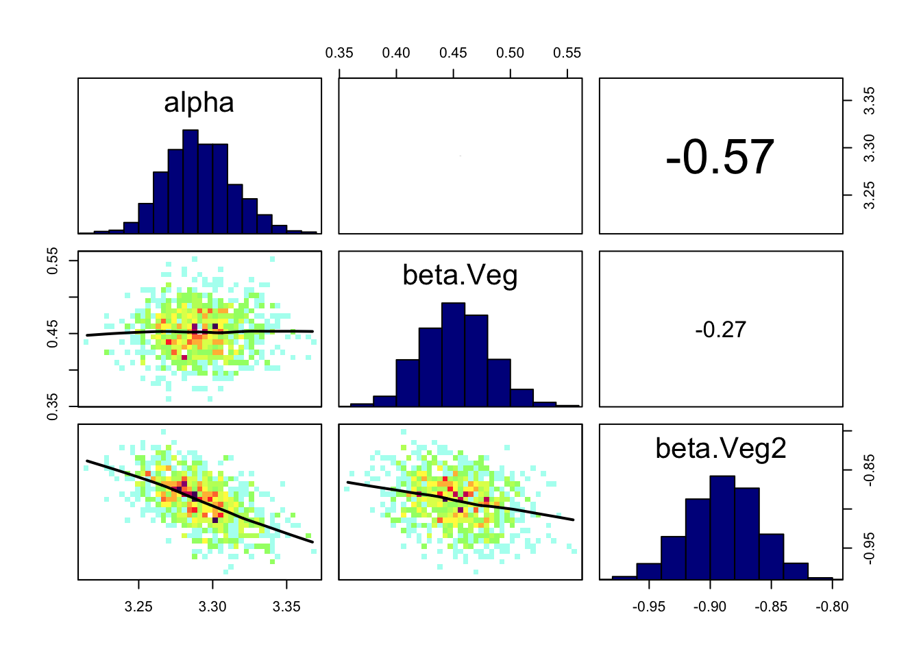
model ="
  model{
  # Likelihood
  for(i in 1:n.dat){
    # poisson model p(y|lambda)
    y[i] ~ dpois(lambda[i])
    # logit link function
    log(lambda[i]) <- mu[i]
    # linear predictor on the log scale
    mu[i] <- alpha + beta.Veg*Veg[i] + beta.Veg2*Veg2[i]
    }
  # Priors
  alpha ~ dnorm(0,0.001)
  beta.Veg  ~ dnorm(0,0.001)
  beta.Veg2 ~ dnorm(0,0.001)

  # Model predictions
  for(i in 1:n.pred){
    y.pred[i] ~ dpois(lambda.pred[i])
    log(lambda.pred[i]) <- mu.pred[i]
    mu.pred[i] <- alpha + beta.Veg*Veg.pred[i] + beta.Veg2*Veg2.pred[i]
    }
  }
 "

###########################################################
# Setting up the JAGS run:

# Set up a list that contains all the necessary data
# Note that for prediction (later used for model checking)
# we here use the original predictor variables.
Model.Data <- list(y = Dat$Count, n.dat = nrow(Dat),
                   Veg = Dat$Veg, Veg2 = Dat$Veg^2,
                   Veg.pred = Dat$Veg, Veg2.pred = Dat$Veg^2,
                   n.pred = nrow(Dat))

# Specify a function to generate inital values for the parameters
inits.fn <- function() list(alpha = rnorm(1,0,1),
                            beta.Veg = rnorm(1,0,1),
                            beta.Veg2 = rnorm(1,0,1))

# Compile the model and run the MCMC for an adaptation (burn-in) phase
jagsModel <- jags.model(file= textConnection(model), data=Model.Data,
                        inits = inits.fn, n.chains = 3, n.adapt= 5000)
Compiling model graph
Resolving undeclared variables
Allocating nodes
Graph information:
Observed stochastic nodes: 200
Unobserved stochastic nodes: 203
Total graph size: 2007
Initializing model# Specify parameters for which posterior samples are saved
para.names <- c('alpha','beta.Veg','beta.Veg2')
# Continue the MCMC runs with sampling
Samples <- coda.samples(jagsModel , variable.names = para.names, n.iter = 5000)
# Statistical summaries of the posterior distributions
summary(Samples)
Iterations = 5001:10000
Thinning interval = 1
Number of chains = 3
Sample size per chain = 5000

1. Empirical mean and standard deviation for each variable,
   plus standard error of the mean:

             Mean      SD  Naive SE Time-series SE
alpha      3.2907 0.02355 0.0001923      0.0003479
beta.Veg   0.4523 0.02929 0.0002392      0.0003554
beta.Veg2 -0.8886 0.02959 0.0002416      0.0004464

2. Quantiles for each variable:

             2.5%     25%    50%     75%   97.5%
alpha      3.2440  3.2750  3.291  3.3066  3.3370
beta.Veg   0.3949  0.4324  0.452  0.4720  0.5110
beta.Veg2 -0.9469 -0.9085 -0.888 -0.8683 -0.8316
# Plot MCMC samples
plot(Samples)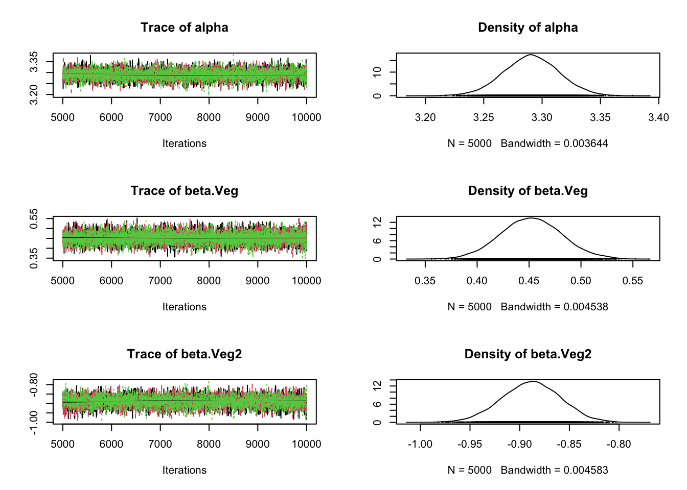
# Check convergence
gelman.diag(Samples)
Potential scale reduction factors:
Point est. Upper C.I.
alpha 1 1
beta.Veg 1 1
beta.Veg2 1 1
Multivariate psrf
1# Correlation plot
correlationPlot(Samples)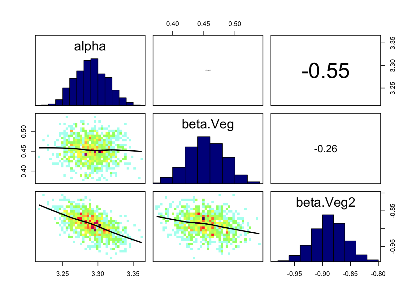
#############################################################
# Sample simulated posterior for lizard counts (y.pred)
Pred.Samples <- coda.samples(jagsModel,
                             variable.names = "y.pred",
                             n.iter = 5000)

# Transform mcmc.list object to a matrix
Pred.Mat <- as.matrix(Pred.Samples)

# Plot Model predictions against data
Pred.Q <- apply(Pred.Mat,2,quantile,prob=c(0.05,0.5,0.95))
plot(Dat$Veg, Dat$Count)
ord <- order(Dat$Veg)
lines(Dat$Veg[ord], Pred.Q['50%',ord],col='blue',lwd=2)
lines(Dat$Veg[ord], Pred.Q['5%',ord],col='blue')
lines(Dat$Veg[ord], Pred.Q['95%',ord],col='blue')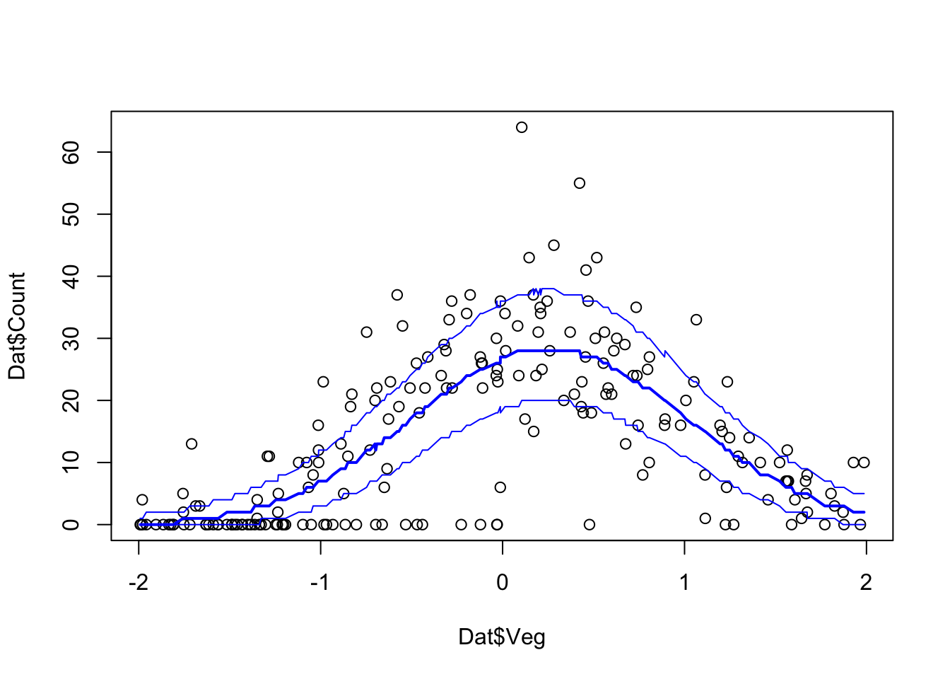
###########################################################
# Model checking with DHARMa
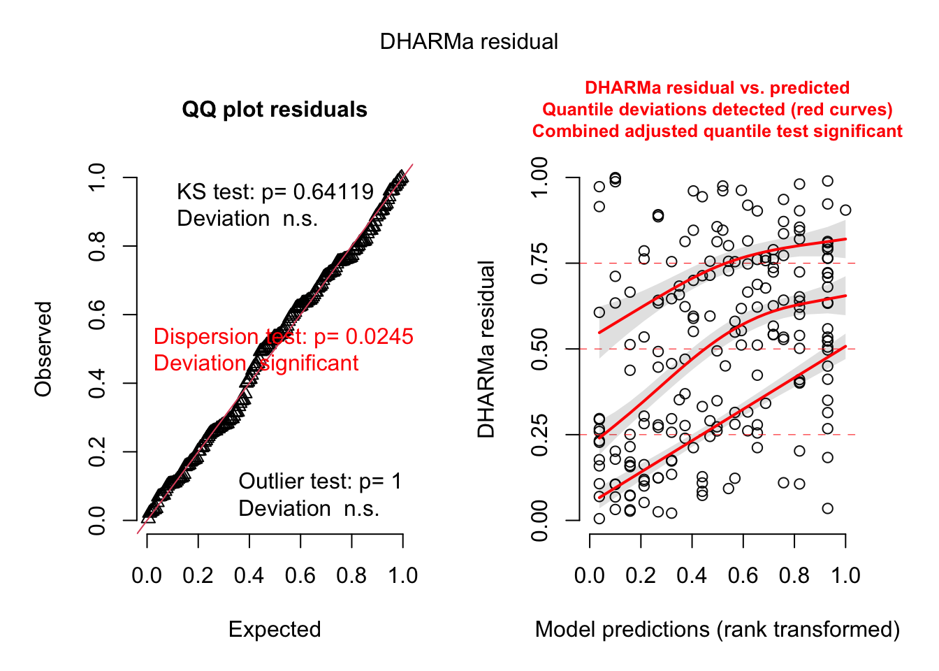
# Create model checking plots
res = createDHARMa(simulatedResponse = t(Pred.Mat),
observedResponse = Dat$Count,
fittedPredictedResponse = apply(Pred.Mat, 2, median),
integer = T)
plot(res)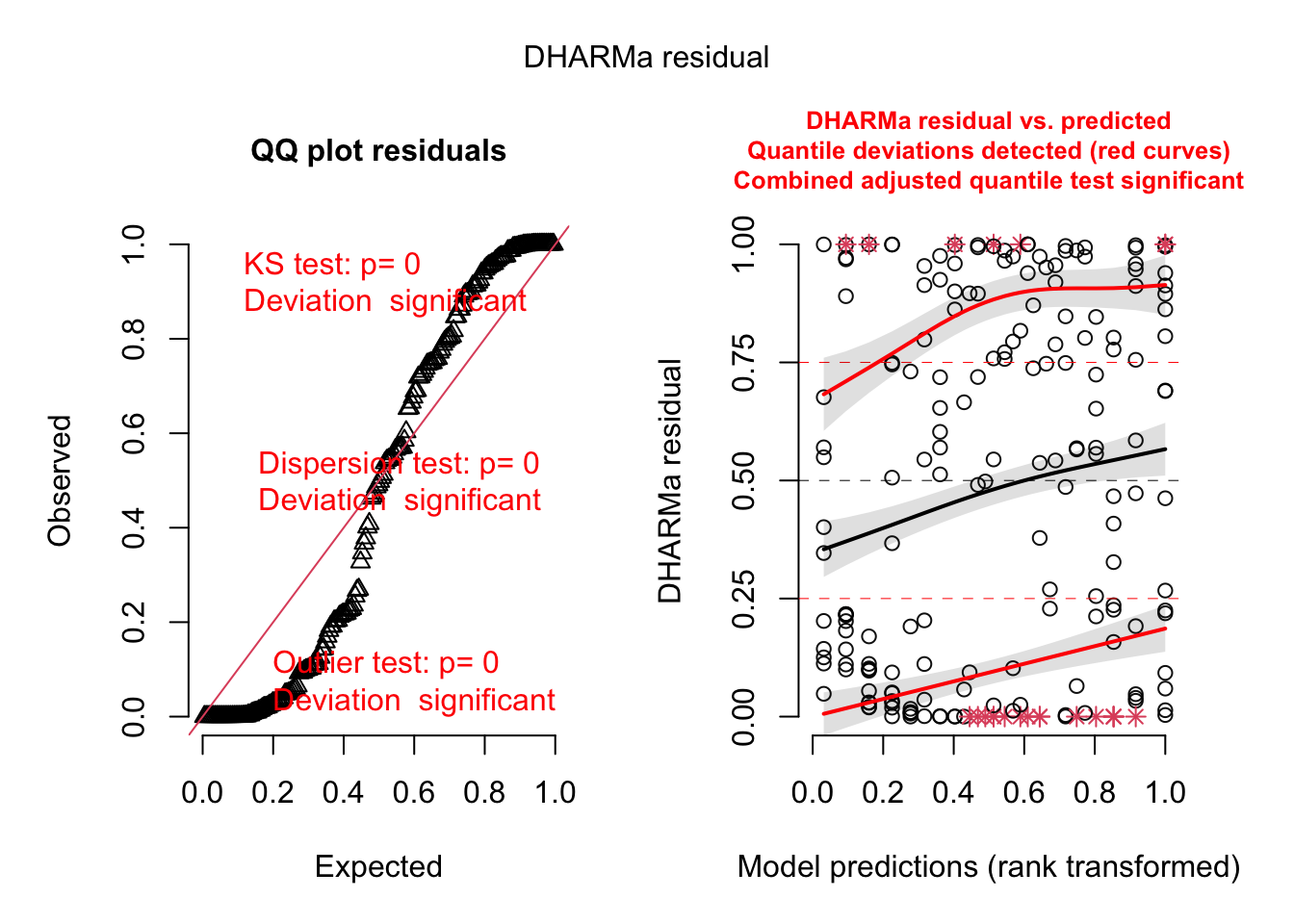
###########################################################model = "
model{
# Likelihood
for(i in 1:n.dat){
# poisson model p(y|lambda)
y[i] ~ dpois(lambda[i])
# logit link function
log(lambda[i]) <- mu[i] + eps[i]
# linear predictor on the log scale
mu[i] <- alpha + beta.Veg*Veg[i] + beta.Veg2*Veg2[i]
# overdispersion error terms
eps[i] ~ dnorm(0,tau.eps)
}
# Priors
alpha ~ dnorm(0,0.001)
beta.Veg ~ dnorm(0,0.001)
beta.Veg2 ~ dnorm(0,0.001)
tau.eps ~ dgamma(0.001,0.001)
# Model predictions
for(i in 1:n.pred){
y.pred[i] ~ dpois(lambda.pred[i])
log(lambda.pred[i]) <- mu.pred[i] + eps.pred[i]
mu.pred[i] <- alpha + beta.Veg*Veg.pred[i] + beta.Veg2*Veg2.pred[i]
eps.pred[i] ~ dnorm(0, tau.eps)
}
}
"
###########################################################
# Setting up the JAGS run:
# Set up a list that contains all the necessary data
# Note that for prediction (later used for model checking)
# we here use the original predictor variables.
Model.Data <- list(y = Dat$Count, n.dat = nrow(Dat),
Veg = Dat$Veg, Veg2 = Dat$Veg^2,
Veg.pred = Dat$Veg, Veg2.pred = Dat$Veg^2,
n.pred = nrow(Dat))
# Specify a function to generate inital values for the parameters
inits.fn <- function() list(alpha = rnorm(1,0,1),
beta.Veg = rnorm(1,0,1),
beta.Veg2 = rnorm(1,0,1),
tau.eps = 1
)
# Compile the model and run the MCMC for an adaptation (burn-in) phase
jagsModel <- jags.model(file= textConnection(model), data=Model.Data,
inits = inits.fn, n.chains = 3, n.adapt= 5000)Compiling model graph
Resolving undeclared variables
Allocating nodes
Graph information:
Observed stochastic nodes: 200
Unobserved stochastic nodes: 604
Total graph size: 3008
Initializing model# Specify parameters for which posterior samples are saved
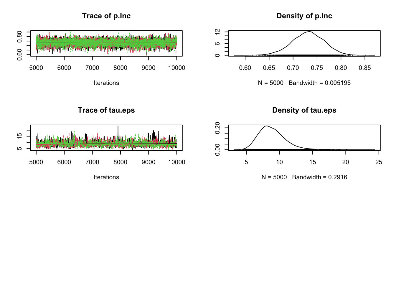
para.names <- c('alpha','beta.Veg','beta.Veg2',
'tau.eps')
# Continue the MCMC runs with sampling
Samples <- coda.samples(jagsModel , variable.names = para.names, n.iter = 5000)
# Statistical summaries of the posterior distributions
summary(Samples)
Iterations = 5001:10000
Thinning interval = 1
Number of chains = 3
Sample size per chain = 5000

1. Empirical mean and standard deviation for each variable,
   plus standard error of the mean:

             Mean      SD  Naive SE Time-series SE
alpha      2.9906 0.11383 0.0009294       0.009623
beta.Veg   0.6682 0.09514 0.0007769       0.004503
beta.Veg2 -0.9983 0.08197 0.0006693       0.004320
tau.eps    0.8520 0.15253 0.0012454       0.004001

2. Quantiles for each variable:

             2.5%     25%     50%     75%   97.5%
alpha      2.7663  2.9132  2.9940  3.0689  3.2019
beta.Veg   0.4889  0.6062  0.6658  0.7264  0.8720
beta.Veg2 -1.1656 -1.0529 -0.9968 -0.9424 -0.8437
tau.eps    0.5894  0.7424  0.8397  0.9474  1.1854
# Plot MCMC samples
plot(Samples)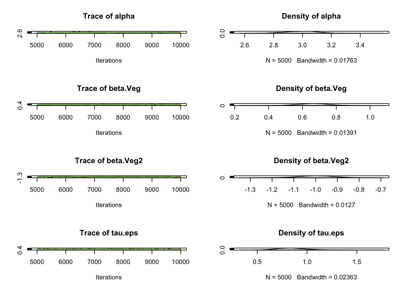
# Check convergence
gelman.diag(Samples)
Potential scale reduction factors:
Point est. Upper C.I.
alpha 1.04 1.14
beta.Veg 1.02 1.06
beta.Veg2 1.02 1.07
tau.eps 1.00 1.00
Multivariate psrf
1.05# Correlation plot
correlationPlot(Samples)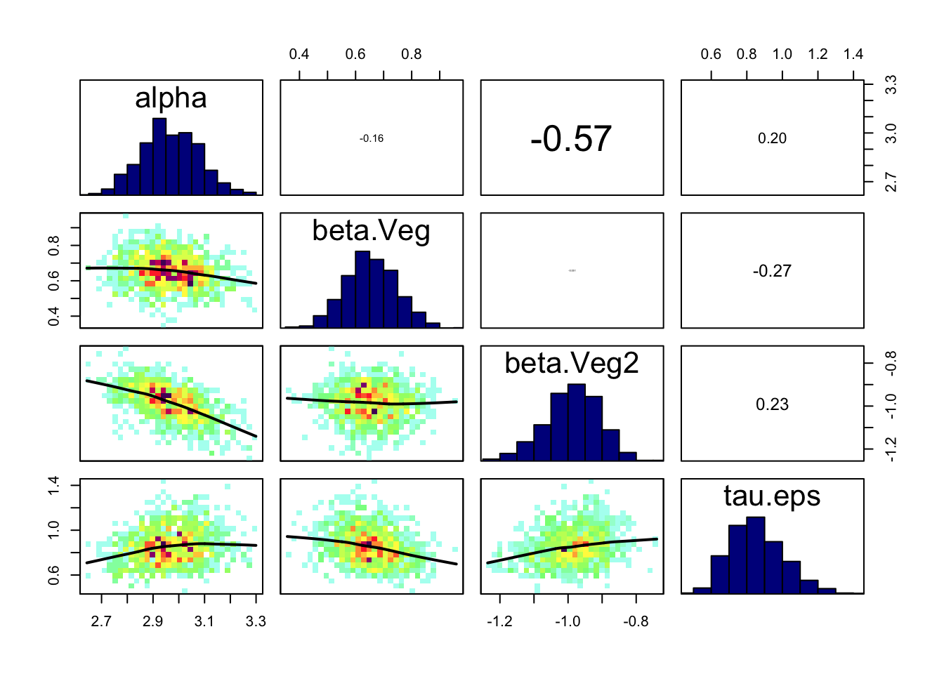
#############################################################
# Sample simulated posterior for lizard counts (y.pred)
Pred.Samples <- coda.samples(jagsModel,
                             variable.names = "y.pred",
                             n.iter = 5000)

# Transform mcmc.list object to a matrix
Pred.Mat <- as.matrix(Pred.Samples)

# Plot Model predictions against data
Pred.Q <- apply(Pred.Mat,2,quantile,prob=c(0.05,0.5,0.95))
plot(Dat$Veg, Dat$Count)
ord <- order(Dat$Veg)
lines(Dat$Veg[ord], Pred.Q['50%',ord],col='blue',lwd=2)
lines(Dat$Veg[ord], Pred.Q['5%',ord],col='blue')
lines(Dat$Veg[ord], Pred.Q['95%',ord],col='blue')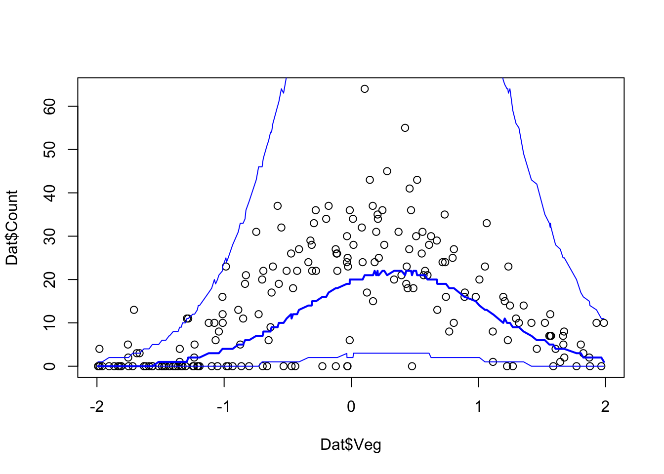
###########################################################
# Model checking with DHARMa

# Create model checking plots
res = createDHARMa(simulatedResponse = t(Pred.Mat),
                   observedResponse = Dat$Count,
                   fittedPredictedResponse = apply(Pred.Mat, 2, median),
                   integer = T)
plot(res)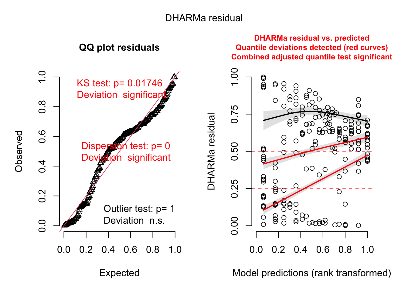
###########################################################model = "
model{
# Likelihood
for(i in 1:n.dat){
# poisson model p(y|lambda)
y[i] ~ dpois(lambda.eff[i])
# effective mean abundance
lambda.eff[i] <- lambda[i] * Inc[i]
# binary variable to indicate occupancy
Inc[i] ~ dbin(p.Inc,1)
# logit link function
log(lambda[i]) <- mu[i] + eps[i]
# linear predictor on the log scale
mu[i] <- alpha + beta.Veg*Veg[i] + beta.Veg2*Veg2[i]
# overdispersion error terms
eps[i] ~ dnorm(0,tau.eps)
}
# Priors
alpha ~ dnorm(0,0.001)
beta.Veg ~ dnorm(0,0.001)
beta.Veg2 ~ dnorm(0,0.001)
tau.eps ~ dgamma(0.001,0.001)
p.Inc ~ dbeta(1,1)
# Model predictions
for(i in 1:n.pred){
y.pred[i] ~ dpois(lambda.eff.pred[i])
lambda.eff.pred[i] <- lambda.pred[i] * Inc.pred[i]
Inc.pred[i] ~ dbin(p.Inc, 1)
log(lambda.pred[i]) <- mu.pred[i] + eps.pred[i]
mu.pred[i] <- alpha + beta.Veg*Veg.pred[i] + beta.Veg2*Veg2.pred[i]
eps.pred[i] ~ dnorm(0, tau.eps)
}
}
"
###########################################################
# Setting up the JAGS run:
# Set up a list that contains all the necessary data
# Note that for prediction (later used for model checking)
# we here use the original predictor variables.
Model.Data <- list(y = Dat$Count, n.dat = nrow(Dat),
Veg = Dat$Veg, Veg2 = Dat$Veg^2,
Veg.pred = Dat$Veg, Veg2.pred = Dat$Veg^2,
n.pred = nrow(Dat))
# Specify a function to generate inital values for the parameters
inits.fn <- function() list(alpha = rnorm(1,0,1),
beta.Veg = rnorm(1,0,1),
beta.Veg2 = rnorm(1,0,1),
tau.eps = 1,
p.Inc = rbeta(1,1,1),
Inc = rep(1,nrow(Dat))
)
# Compile the model and run the MCMC for an adaptation (burn-in) phase
jagsModel <- jags.model(file= textConnection(model), data=Model.Data,
inits = inits.fn, n.chains = 3, n.adapt= 5000)Compiling model graph
Resolving undeclared variables
Allocating nodes
Graph information:
Observed stochastic nodes: 200
Unobserved stochastic nodes: 1005
Total graph size: 3810
Initializing model# Specify parameters for which posterior samples are saved
para.names <- c('alpha','beta.Veg','beta.Veg2',
'tau.eps','p.Inc')
# Continue the MCMC runs with sampling
Samples <- coda.samples(jagsModel , variable.names = para.names, n.iter = 5000)
# Statistical summaries of the posterior distributions
summary(Samples)
Iterations = 5001:10000
Thinning interval = 1
Number of chains = 3
Sample size per chain = 5000

1. Empirical mean and standard deviation for each variable,
   plus standard error of the mean:

             Mean      SD  Naive SE Time-series SE
alpha      3.3355 0.04714 0.0003849       0.001581
beta.Veg   0.2093 0.05037 0.0004113       0.001275
beta.Veg2 -0.6882 0.04761 0.0003887       0.001402
p.Inc      0.7313 0.03353 0.0002738       0.000445
tau.eps    8.8435 1.96433 0.0160387       0.057017

2. Quantiles for each variable:

             2.5%     25%     50%     75%   97.5%
alpha      3.2399  3.3044  3.3362  3.3675  3.4253
beta.Veg   0.1130  0.1754  0.2086  0.2432  0.3099
beta.Veg2 -0.7839 -0.7199 -0.6879 -0.6558 -0.5958
p.Inc      0.6629  0.7091  0.7320  0.7542  0.7949
tau.eps    5.6401  7.4571  8.6237  9.9795 13.2890
# Plot MCMC samples
plot(Samples)
# Check convergence
gelman.diag(Samples)
Potential scale reduction factors:
Point est. Upper C.I.
alpha 1 1.00
beta.Veg 1 1.01
beta.Veg2 1 1.01
p.Inc 1 1.00
tau.eps 1 1.01
Multivariate psrf
1.01# Correlation plot
correlationPlot(Samples)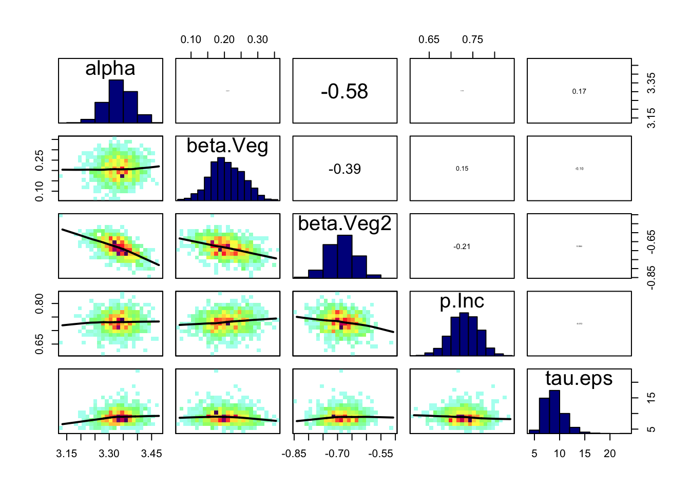
#############################################################
# Sample simulated posterior for lizard counts (y.pred)
Pred.Samples <- coda.samples(jagsModel,
                             variable.names = "y.pred",
                             n.iter = 5000)

# Transform mcmc.list object to a matrix
Pred.Mat <- as.matrix(Pred.Samples)

# Plot Model predictions against data
Pred.Q <- apply(Pred.Mat,2,quantile,prob=c(0.05,0.5,0.95))
plot(Dat$Veg, Dat$Count)
ord <- order(Dat$Veg)
lines(Dat$Veg[ord], Pred.Q['50%',ord],col='blue',lwd=2)
lines(Dat$Veg[ord], Pred.Q['5%',ord],col='blue')
lines(Dat$Veg[ord], Pred.Q['95%',ord],col='blue')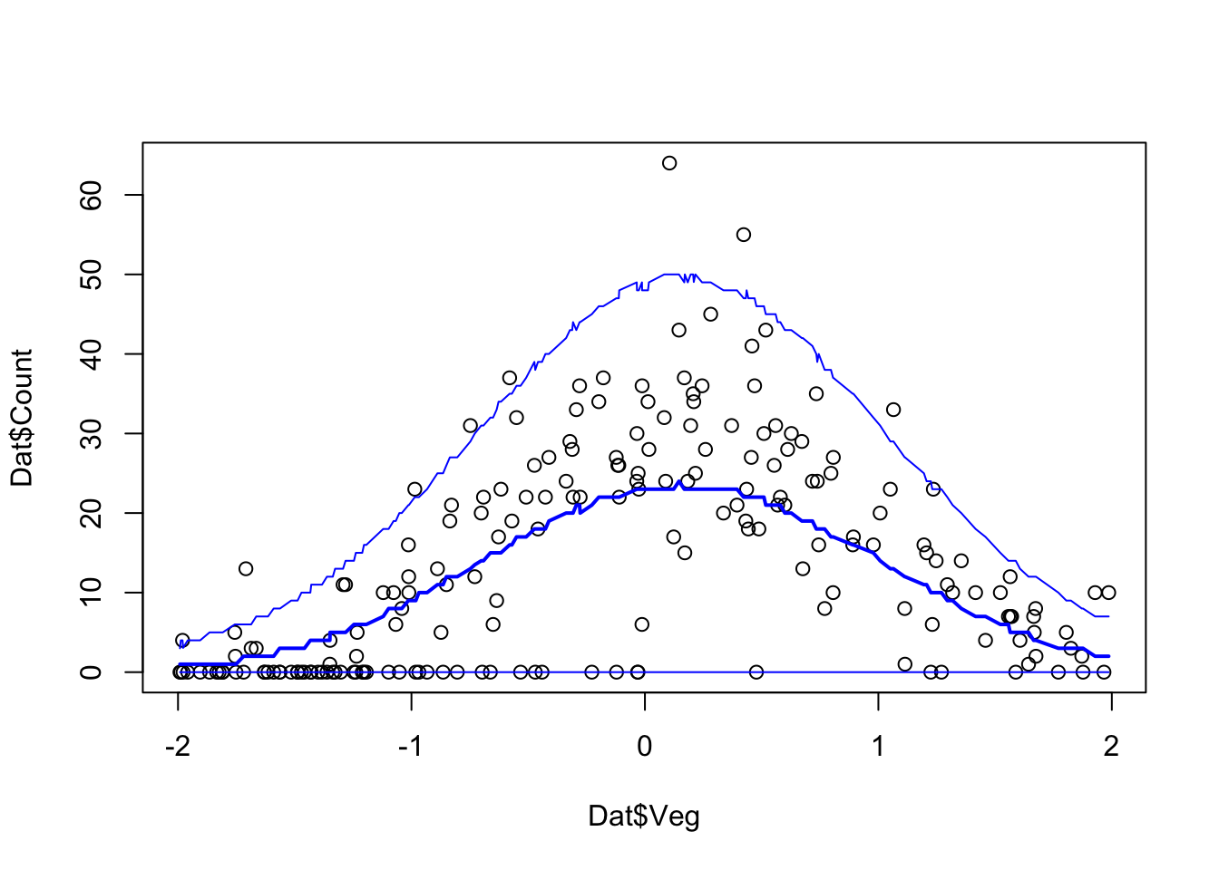
###########################################################
# Model checking with DHARMa

# Create model checking plots
res = createDHARMa(simulatedResponse = t(Pred.Mat),
                   observedResponse = Dat$Count,
                   fittedPredictedResponse = apply(Pred.Mat, 2, median),
                   integer = T)
plot(res)