[9]{.chapter-number}  [Occupancy models]{.chapter-title}

9 Occupancy models

library(EcoData)
library(effects)

Loading required package: carData

lattice theme set by effectsTheme()
See ?effectsTheme for details.

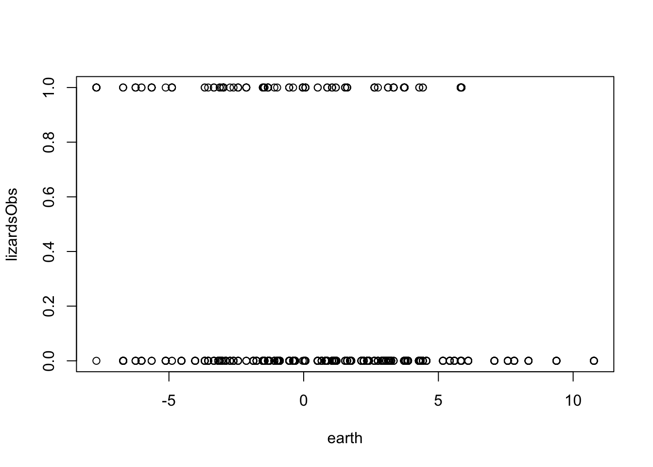
plot(lizardsObs ~ earth , data = volcanoisland)

fit<- glm(lizardsObs ~ earth + windObs , data = volcanoisland, family = binomial)

Warning: glm.fit: fitted probabilities numerically 0 or 1 occurred

summary(fit)


Call:
glm(formula = lizardsObs ~ earth + windObs, family = binomial, 
    data = volcanoisland)

Deviance Residuals: 
     Min        1Q    Median        3Q       Max  
-2.20221  -0.50521  -0.15234  -0.00544   3.03979  

Coefficients:
            Estimate Std. Error z value Pr(>|z|)    
(Intercept)  1.16640    0.21592   5.402 6.59e-08 ***
earth       -0.21692    0.02982  -7.273 3.51e-13 ***
windObs     -0.61135    0.05763 -10.608  < 2e-16 ***
---
Signif. codes:  0 '***' 0.001 '**' 0.01 '*' 0.05 '.' 0.1 ' ' 1

(Dispersion parameter for binomial family taken to be 1)

    Null deviance: 889.22  on 999  degrees of freedom
Residual deviance: 562.65  on 997  degrees of freedom
AIC: 568.65

Number of Fisher Scoring iterations: 8

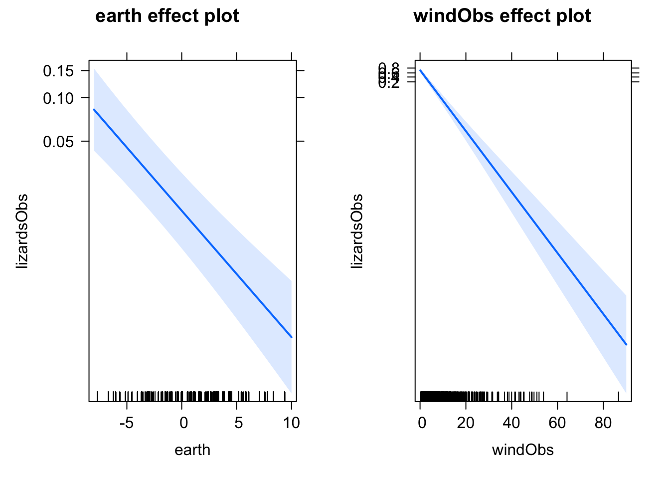
plot(allEffects(fit))

However, there is something wrong with the model

library(DHARMa)

This is DHARMa 0.4.6. For overview type '?DHARMa'. For recent changes, type news(package = 'DHARMa')

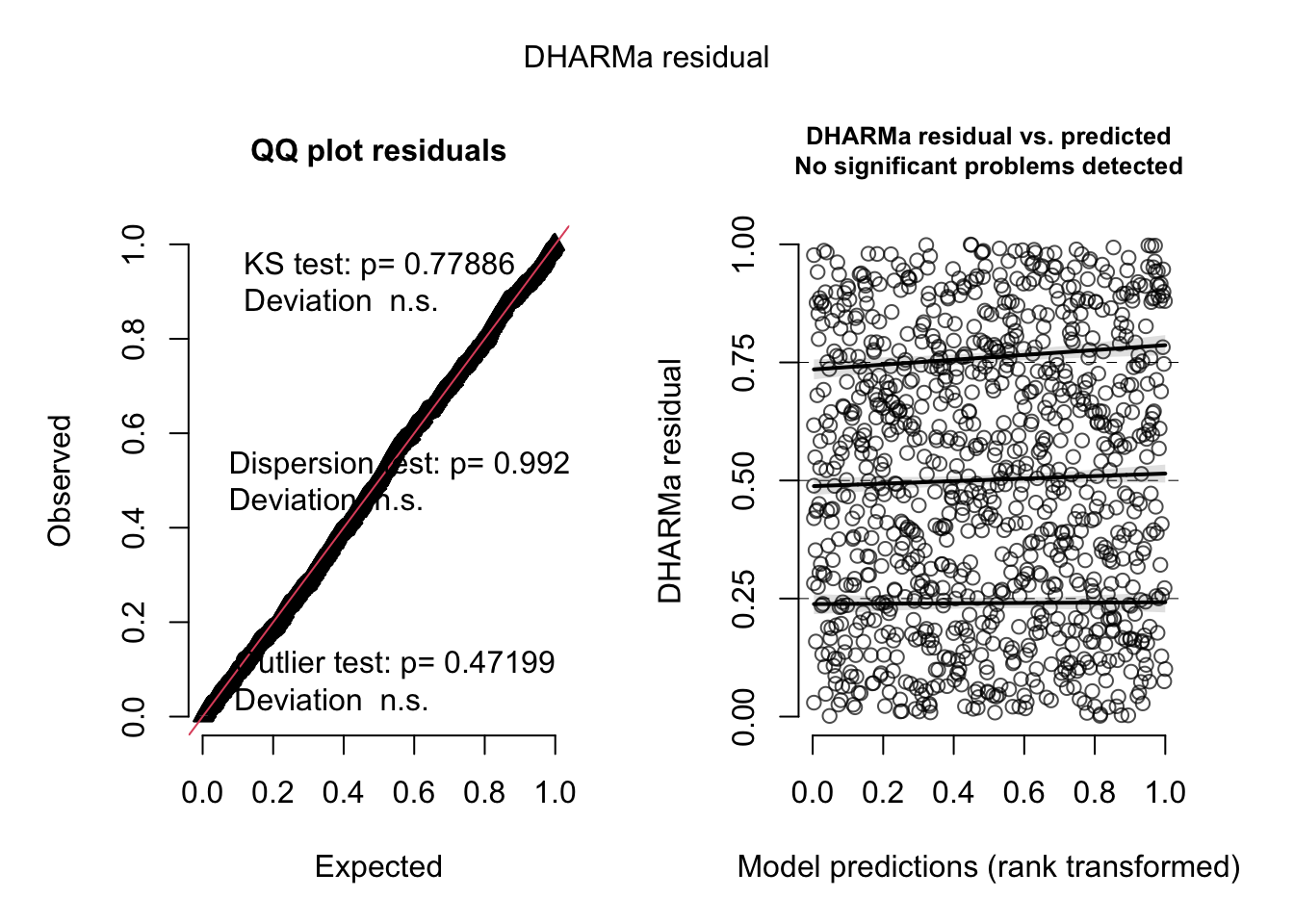
res <- simulateResiduals(fit)
plot(res)

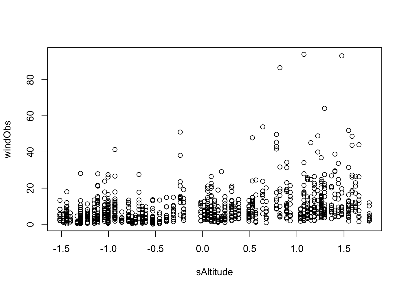
Suspicion - the lizards atually depend on the altitude, but they don’t like wind and therefore hide when there is a lot of wind, and wind also correlates with altitude.

plot(windObs ~ sAltitude, data = volcanoisland)

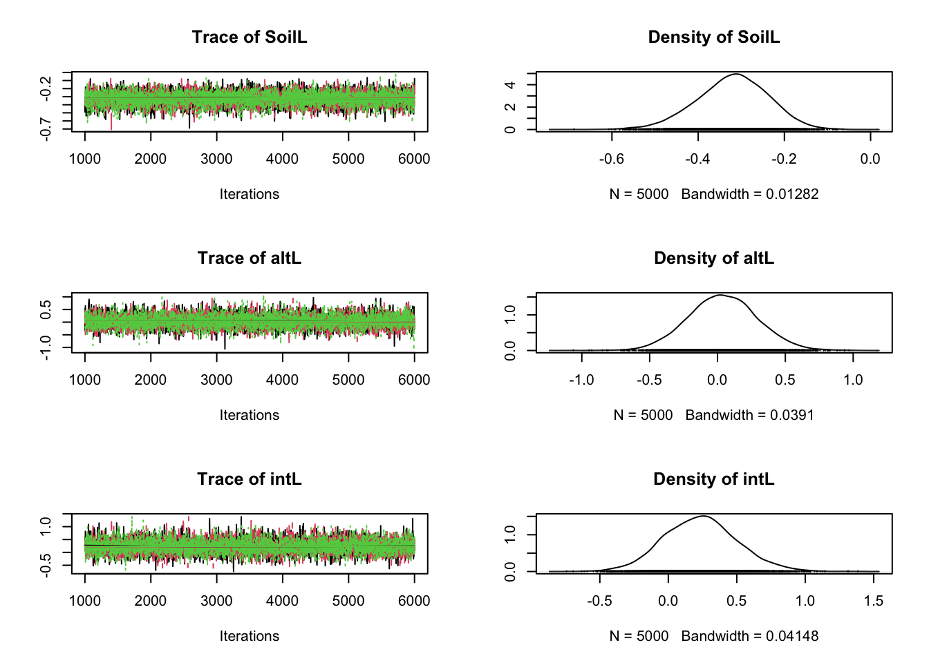
Could we find out what’s the true effect of the environmental predictors? let’s build an occupancy model where we model the true presence of the lizzard as a latent variable.

library(rjags)

Loading required package: coda

Linked to JAGS 4.3.0

Loaded modules: basemod,bugs

Data = list(WindObs = log(volcanoisland$windObs),
            Altitude = volcanoisland$sAltitude[seq(1, 999, by = 10)],
            SoilPlot = unique(volcanoisland$earth),
            LizzardObs =volcanoisland$lizardsObs,
            plot = as.numeric(volcanoisland$plot),
            nobs = nrow(volcanoisland),
            nplots = length(unique(volcanoisland$plot)))


modelCode = "
model{

  # Likelihood
  for(i in 1:nobs){

    LizzardObs[i] ~ dbern(ObservationProb[i] *  LizzardTrue[plot[i]])
    logit(ObservationProb[i]) <- intO + windO * WindObs[i]

  }

  for(i in 1:nplots){
    LizzardTrue[i] ~ dbern(LizzardSuitability[i])
    logit(LizzardSuitability[i]) <- intL+ SoilL*SoilPlot[i] + altL * Altitude[i]
  }

  # Prior distributions
  intO ~ dnorm(0,0.001)
  windO ~ dnorm(0,0.001)
  intL ~ dnorm(0,0.001)
  SoilL ~ dnorm(0,0.001)
  altL ~ dnorm(0,0.001)

  # posterior predictive simulations

  # Likelihood
  for(i in 1:nobs){
    LizzardObsSim[i] ~ dbern(ObservationProb[i] *  LizzardTrueSim[plot[i]])
  }
  for(i in 1:nplots){
    LizzardTrueSim[i] ~ dbern(LizzardSuitability[i])
  }

}
"

inits.fn <- function() list(LizzardTrue = rep(1,100))
jagsModel <- jags.model(file= textConnection(modelCode), inits = inits.fn, data=Data, n.chains = 3)

Compiling model graph
   Resolving undeclared variables
   Allocating nodes
Graph information:
   Observed stochastic nodes: 1000
   Unobserved stochastic nodes: 1205
   Total graph size: 9771

Initializing model

para.names <- c("intO","windO","intL", "SoilL", "altL")
Samples <- coda.samples(jagsModel, variable.names = para.names, n.iter = 5000)
plot(Samples)

summary(Samples)


Iterations = 1001:6000
Thinning interval = 1 
Number of chains = 3 
Sample size per chain = 5000 

1. Empirical mean and standard deviation for each variable,
   plus standard error of the mean:

          Mean      SD  Naive SE Time-series SE
SoilL -0.32036 0.08307 0.0006783       0.001047
altL   0.04013 0.25479 0.0020803       0.003181
intL   0.23622 0.26860 0.0021931       0.003652
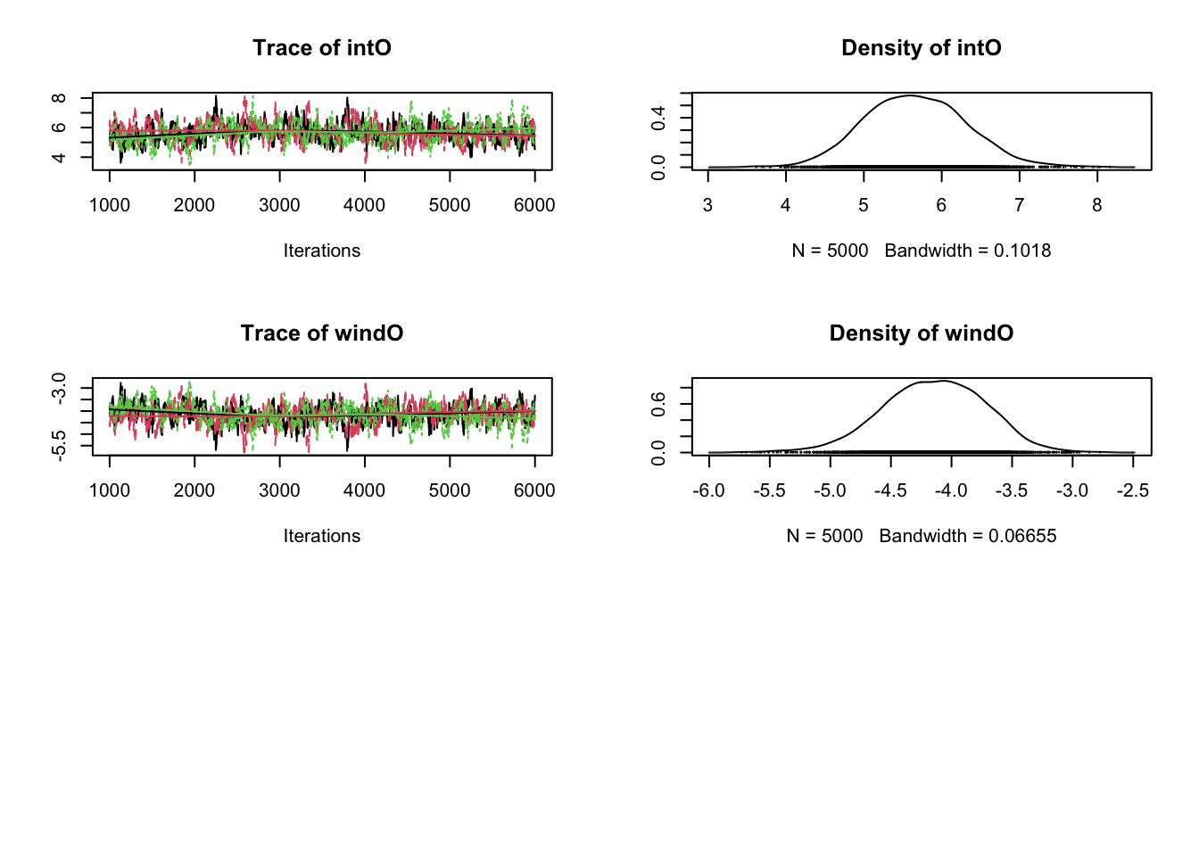
intO   5.66535 0.65717 0.0053657       0.038296
windO -4.14582 0.42957 0.0035074       0.025122

2. Quantiles for each variable:

         2.5%      25%      50%     75%   97.5%
SoilL -0.4928 -0.37404 -0.31692 -0.2632 -0.1663
altL  -0.4540 -0.13044  0.03736  0.2078  0.5453
intL  -0.2759  0.05005  0.23318  0.4088  0.7863
intO   4.4430  5.20658  5.65008  6.1011  6.9961
windO -5.0138 -4.43041 -4.13413 -3.8423 -3.3544

dic = dic = dic.samples(jagsModel, n.iter = 5000, type = "pD")
dic

Mean deviance:  261 
penalty NaN 
Penalized deviance: NaN

Inspecting the occupancy results

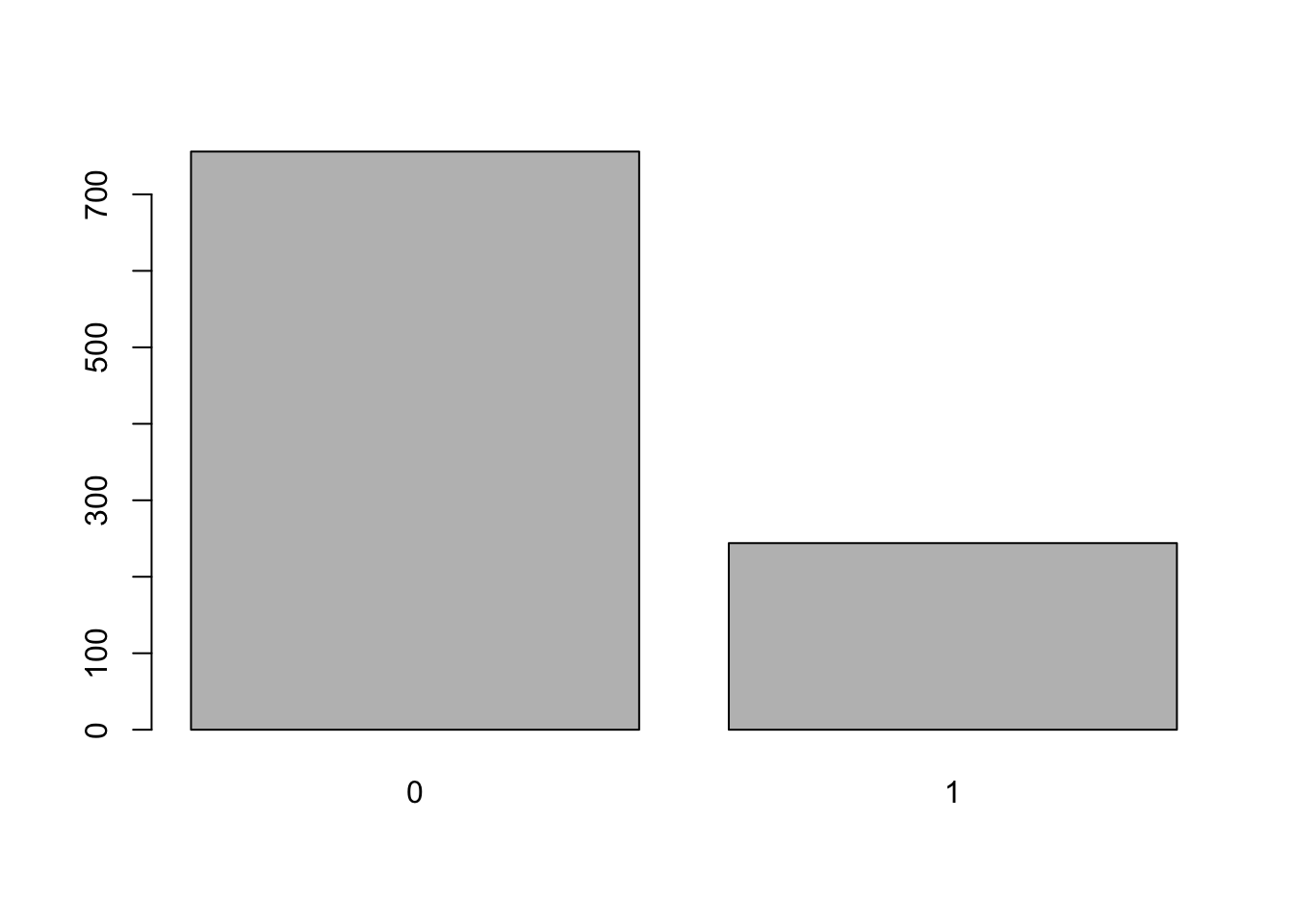
para.names <- c("LizzardTrue")
Samples <- coda.samples(jagsModel, variable.names = para.names, n.iter = 5000)

library(BayesianTools)
x = getSample(Samples)

# there was no Lizard observed on plot 3 on all 10 replicates
volcanoisland$lizardsObs[21:30]

 [1] 0 0 0 0 0 0 0 0 0 0

# Still, occupancy probability that the species is there is 22 percent
barplot(table(x[,3]))

para.names <- c("LizzardSuitability")
Samples <- coda.samples(jagsModel, variable.names = para.names, n.iter = 5000)
x = getSample(Samples)
S=x
Suitability = apply(S,2,mean)
uncertaintyS = apply(S,2,sd)

x = volcanoisland$x[seq(1, 999, by = 10)]
y = volcanoisland$y[seq(1, 999, by = 10)]

par(mfrow = c(1,2))

plot(x,y, cex = Suitability)
plot(x,y, cex = uncertaintyS)

Checking residuals of this model

para.names <- c("LizzardObsSim")
Samples <- coda.samples(jagsModel, variable.names = para.names, n.iter = 5000)

library(DHARMa)
x = getSample(Samples)


sim = createDHARMa(simulatedResponse = t(x), observedResponse = volcanoisland$lizardsObs, fittedPredictedResponse = apply(x, 2, mean), integerResponse = T)
plot(sim)

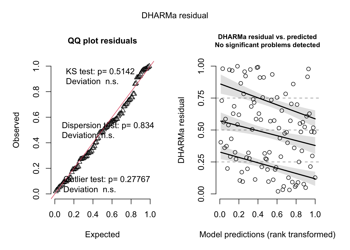
# fix for a bug in DHARMa, will be corrected
sim$simulatedResponse = t(x)
sim$refit = F
sim$integerResponse = T

res2 = recalculateResiduals(sim, group = as.factor(volcanoisland$plot))

plot(res2)

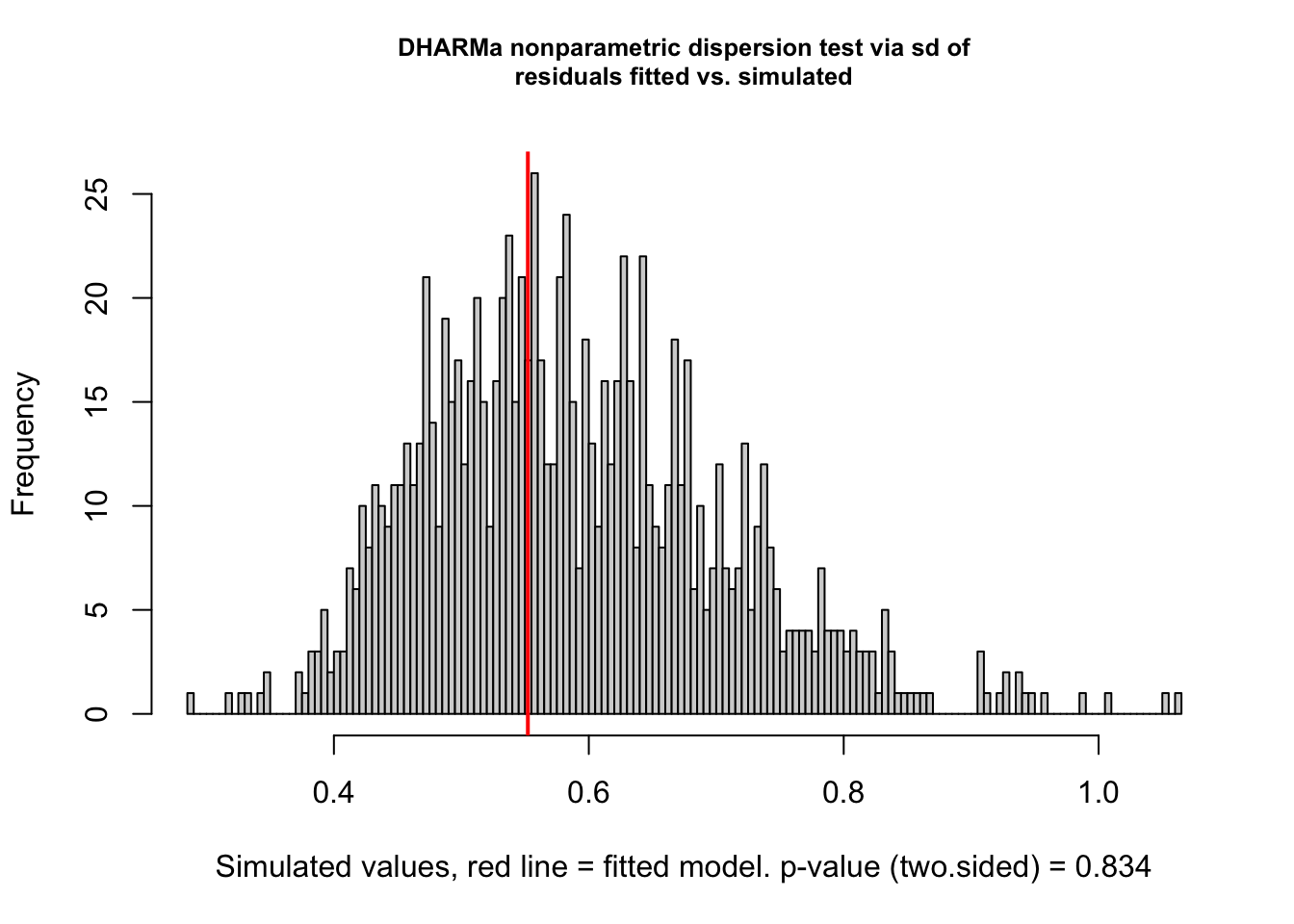
testDispersion(res2)


    DHARMa nonparametric dispersion test via sd of residuals fitted vs.
    simulated

data:  simulationOutput
dispersion = 0.93804, p-value = 0.834
alternative hypothesis: two.sided

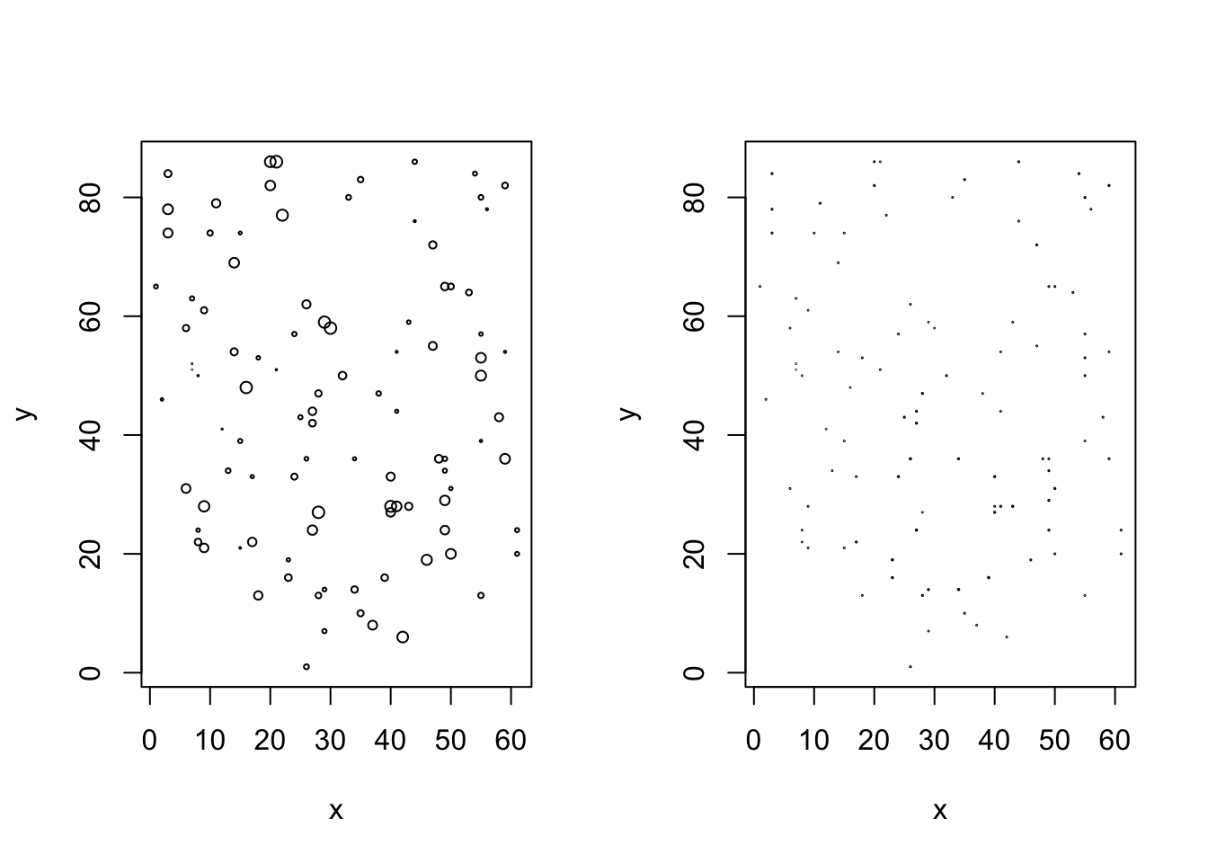
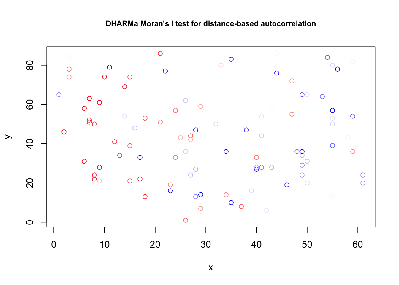
x = volcanoisland$x[seq(1, 999, by = 10)]
y = volcanoisland$y[seq(1, 999, by = 10)]

testSpatialAutocorrelation(res2, x = x, y = y)


    DHARMa Moran's I test for distance-based autocorrelation

data:  res2
observed = 0.115750, expected = -0.010101, sd = 0.017233, p-value =
2.818e-13
alternative hypothesis: Distance-based autocorrelation