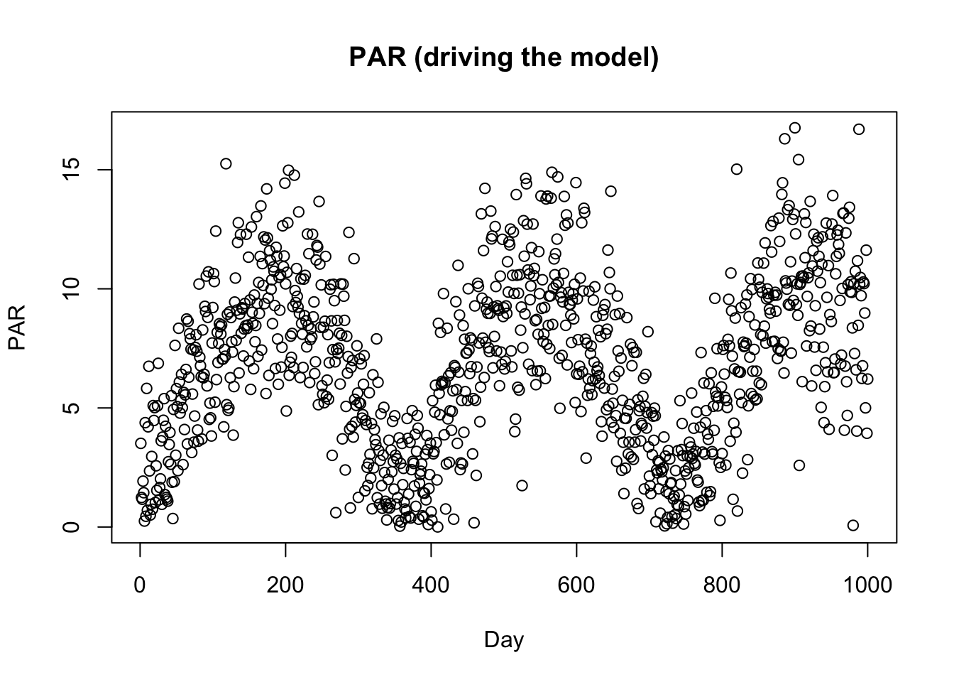
[14]{.chapter-number}  [Process-based models]{.chapter-title}

14 Process-based models

library(BayesianTools)

# Create input data for the model
PAR <- VSEMcreatePAR(1:1000)
plot(PAR, main = "PAR (driving the model)", xlab = "Day")

# load reference parameter definition (upper, lower prior)
refPars <- VSEMgetDefaults()
# this adds one additional parameter for the likelihood standard deviation (see below)
refPars[12,] <- c(2, 0.1, 4) 
rownames(refPars)[12] <- "error-sd"
head(refPars)

           best lower upper
KEXT      0.500 2e-01 1e+00
LAR       1.500 2e-01 3e+00
LUE       0.002 5e-04 4e-03
GAMMA     0.400 2e-01 6e-01
tauV   1440.000 5e+02 3e+03
tauS  27370.000 4e+03 5e+04

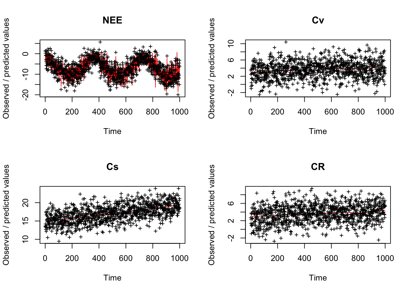
# create some simulated test data 
# generally recommended to start with simulated data before moving to real data
referenceData <- VSEM(refPars$best[1:11], PAR) # model predictions with reference parameters  
referenceData[,1] = 1000 * referenceData[,1] 
# this adds the error - needs to conform to the error definition in the likelihood
obs <- referenceData + rnorm(length(referenceData), sd = refPars$best[12])
oldpar <- par(mfrow = c(2,2))
for (i in 1:4) plotTimeSeries(observed = obs[,i], 
                              predicted = referenceData[,i], main = colnames(referenceData)[i])

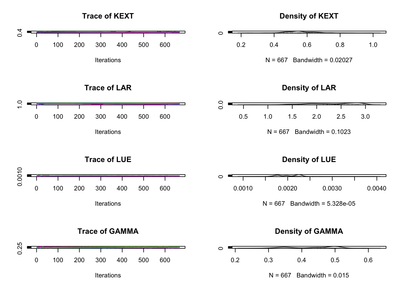
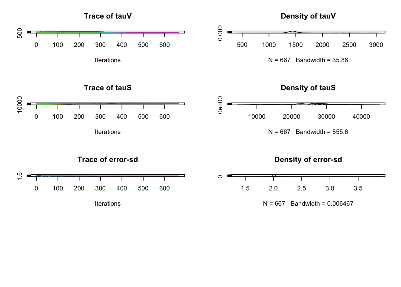
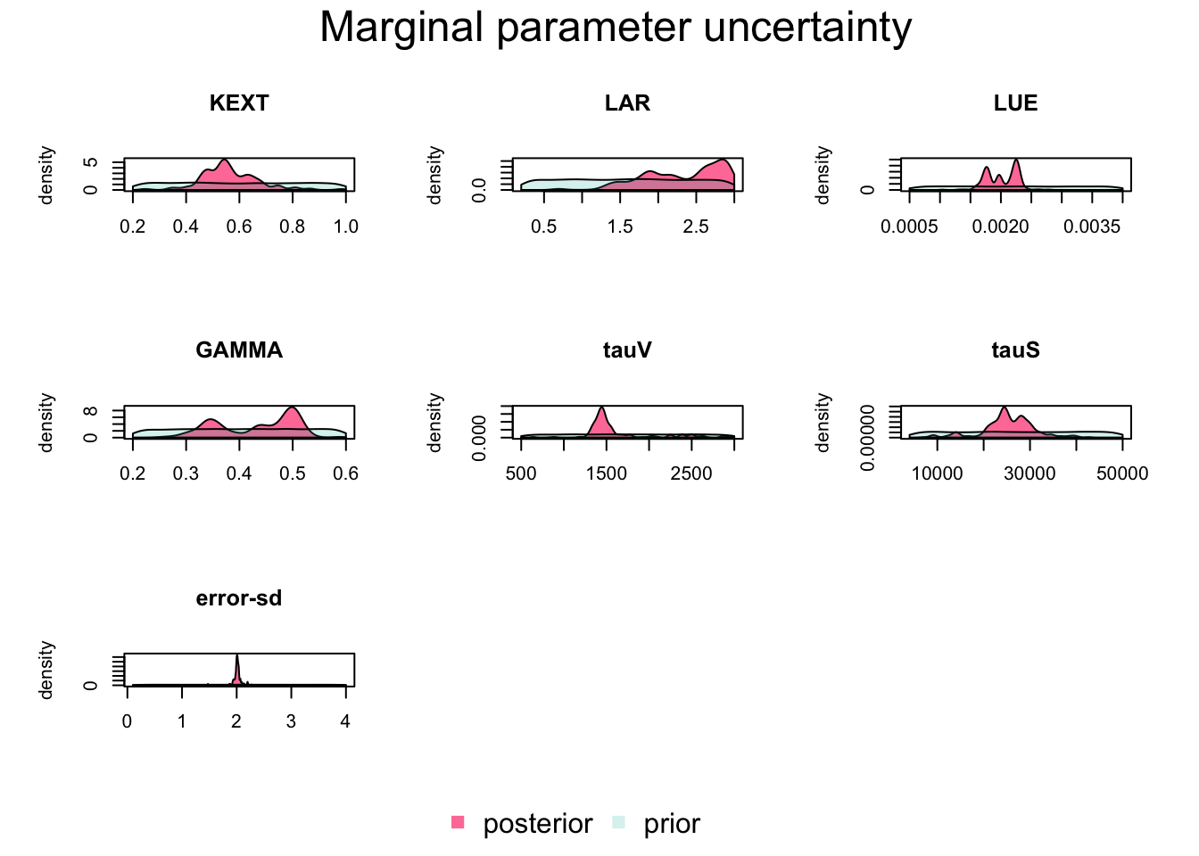
# Best to program in a way that we can choose easily which parameters to calibrate
parSel = c(1:6, 12)

# here is the likelihood 
likelihood <- function(par, sum = TRUE){
  # set parameters that are not calibrated on default values 
  x = refPars$best
  x[parSel] = par
  predicted <- VSEM(x[1:11], PAR) # replace here VSEM with your model 
  predicted[,1] = 1000 * predicted[,1] # this is just rescaling
  diff <- c(predicted[,1:4] - obs[,1:4]) # difference betweeno observed and predicted
  # univariate normal likelihood. Note that there is a parameter involved here that is fit
  llValues <- dnorm(diff, sd = x[12], log = TRUE)  
  if (sum == FALSE) return(llValues)
  else return(sum(llValues))
}

# optional, you can also directly provide lower, upper in the createBayesianSetup, see help
prior <- createUniformPrior(lower = refPars$lower[parSel], 
                            upper = refPars$upper[parSel], best = refPars$best[parSel])

bayesianSetup <- createBayesianSetup(likelihood, prior, names = rownames(refPars)[parSel])

# settings for the sampler, iterations should be increased for real applicatoin
settings <- list(iterations = 2000, nrChains = 2)

out <- runMCMC(bayesianSetup = bayesianSetup, sampler = "DEzs", settings = settings)


 Running DEzs-MCMC, chain  1 iteration 300 of 2001 . Current logp  -8566.156 -8499.593 -8507.241 . Please wait! 

 Running DEzs-MCMC, chain  1 iteration 600 of 2001 . Current logp  -8489.945 -8489.103 -8485.902 . Please wait! 

 Running DEzs-MCMC, chain  1 iteration 900 of 2001 . Current logp  -8486.072 -8489.803 -8489.643 . Please wait! 

 Running DEzs-MCMC, chain  1 iteration 1200 of 2001 . Current logp  -8486.468 -8485.746 -8485.014 . Please wait! 

 Running DEzs-MCMC, chain  1 iteration 1500 of 2001 . Current logp  -8485.923 -8491.022 -8486.336 . Please wait! 

 Running DEzs-MCMC, chain  1 iteration 1800 of 2001 . Current logp  -8485.298 -8487.846 -8484.556 . Please wait! 

 Running DEzs-MCMC, chain  1 iteration 2001 of 2001 . Current logp  -8485.874 -8485.425 -8487.278 . Please wait!

runMCMC terminated after 1.579seconds


 Running DEzs-MCMC, chain  2 iteration 300 of 2001 . Current logp  -8561.552 -8563.564 -8569.686 . Please wait! 

 Running DEzs-MCMC, chain  2 iteration 600 of 2001 . Current logp  -8538.887 -8538.977 -8546.54 . Please wait! 

 Running DEzs-MCMC, chain  2 iteration 900 of 2001 . Current logp  -8502.444 -8491.463 -8522.535 . Please wait! 

 Running DEzs-MCMC, chain  2 iteration 1200 of 2001 . Current logp  -8486.893 -8487.119 -8487.553 . Please wait! 

 Running DEzs-MCMC, chain  2 iteration 1500 of 2001 . Current logp  -8487.805 -8486.57 -8484.996 . Please wait! 

 Running DEzs-MCMC, chain  2 iteration 1800 of 2001 . Current logp  -8484.447 -8487.071 -8488.836 . Please wait! 

 Running DEzs-MCMC, chain  2 iteration 2001 of 2001 . Current logp  -8485.458 -8488.215 -8485.654 . Please wait!

runMCMC terminated after 1.828seconds

plot(out)

summary(out)

# # # # # # # # # # # # # # # # # # # # # # # # # 
## MCMC chain summary ## 
# # # # # # # # # # # # # # # # # # # # # # # # # 
 
# MCMC sampler:  DEzs 
# Nr. Chains:  6 
# Iterations per chain:  667 
# Rejection rate:  0.909 
# Effective sample size:  72 
# Runtime:  3.407  sec. 
 
# Parameters
           psf       MAP      2.5%    median     97.5%
KEXT     1.210     0.438     0.364     0.549     0.807
LAR      2.261     2.708     1.358     2.433     2.965
LUE      5.705     0.002     0.002     0.002     0.002
GAMMA    6.758     0.515     0.298     0.450     0.527
tauV     1.189  1475.404  1190.045  1471.547  2867.823
tauS     1.425 31318.063 12105.862 25200.275 37808.067
error-sd 1.072     2.016     1.873     2.012     2.202

## DIC:  17263.1 
## Convergence 
 Gelman Rubin multivariate psrf:  8.746 
 
## Correlations 
           KEXT    LAR    LUE  GAMMA   tauV   tauS error-sd
KEXT      1.000 -0.228 -0.345 -0.286  0.333  0.050   -0.102
LAR      -0.228  1.000  0.612  0.592 -0.129 -0.052    0.040
LUE      -0.345  0.612  1.000  0.890  0.029  0.067    0.108
GAMMA    -0.286  0.592  0.890  1.000  0.080  0.265   -0.017
tauV      0.333 -0.129  0.029  0.080  1.000  0.170   -0.057
tauS      0.050 -0.052  0.067  0.265  0.170  1.000   -0.338
error-sd -0.102  0.040  0.108 -0.017 -0.057 -0.338    1.000

marginalPlot(out)

gelmanDiagnostics(out) # should be below 1.05 for all parameters to demonstrate convergence

Potential scale reduction factors:

         Point est. Upper C.I.
KEXT           1.21       1.51
LAR            2.26       3.84
LUE            5.70       9.63
GAMMA          6.76      11.61
tauV           1.19       1.50
tauS           1.42       2.02
error-sd       1.07       1.17

Multivariate psrf

8.75

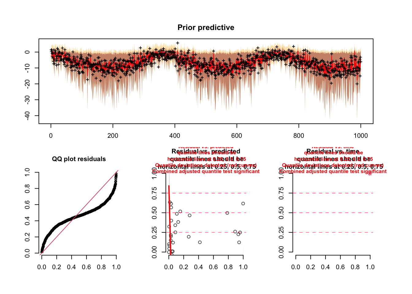
# Posterior predictive simulations

# Create a prediction function
createPredictions <- function(par){
  # set the parameters that are not calibrated on default values 
  x = refPars$best
  x[parSel] = par
  predicted <- VSEM(x[1:11], PAR) # replace here VSEM with your model 
  return(predicted[,1] * 1000)
}

# Create an error function
createError <- function(mean, par){
  return(rnorm(length(mean), mean = mean, sd = par[7]))
}

# plot prior predictive distribution and prior predictive simulations
plotTimeSeriesResults(sampler = out, model = createPredictions, observed = obs[,1],
                      error = createError, prior = TRUE, main = "Prior predictive")

DHARMa::plotTimeSeriesResults called with posterior predictive (residual) diagnostics. Type vignette("DHARMa", package="DHARMa") for a guide on how to interpret these plots

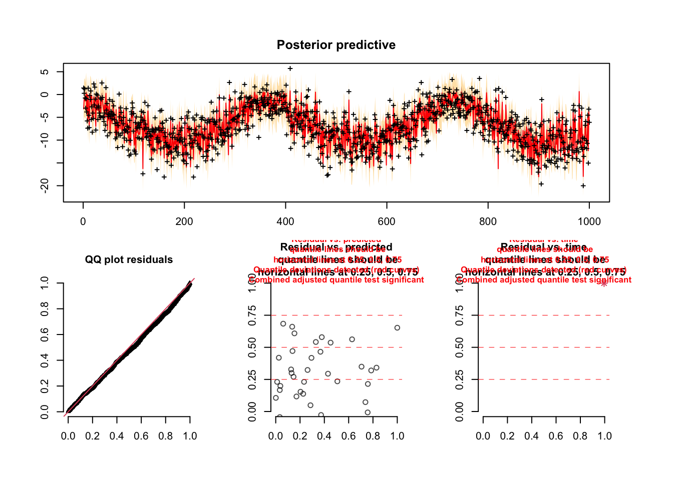
# plot posterior predictive distribution and posterior predictive simulations
plotTimeSeriesResults(sampler = out, model = createPredictions, observed = obs[,1],
                      error = createError, main = "Posterior predictive")

DHARMa::plotTimeSeriesResults called with posterior predictive (residual) diagnostics. Type vignette("DHARMa", package="DHARMa") for a guide on how to interpret these plots