meanSize <- 10
trueLogSd <- 1
sampleSize <- 500
truevalues = rexp(rate = 1/meanSize, n = sampleSize)
observations = rlnorm(n = length(truevalues), mean = log(truevalues), sd = trueLogSd)8 Error in variable models
8.1 Regression dillution in distribution estimates
8.1.1 Creation of the data
Assume we observe data from an ecological system that creates an exponential size distribution (e.g. tree sizes, see Taubert, F.; Hartig, F.; Dobner, H.-J. & Huth, A. (2013) On the Challenge of Fitting Tree Size Distributions in Ecology. PLoS ONE, 8, e58036-), but our measurments are performed with a substantial lognormal observation error
Plotting true and observed data
maxV <- ceiling(max(observations,truevalues))
counts <- rbind(
  obs = hist(observations, breaks = 0:maxV, plot = F)$counts,
  true = hist(truevalues, breaks = 0:maxV, plot = F)$counts
)
barplot(log(t(counts)+1), beside=T)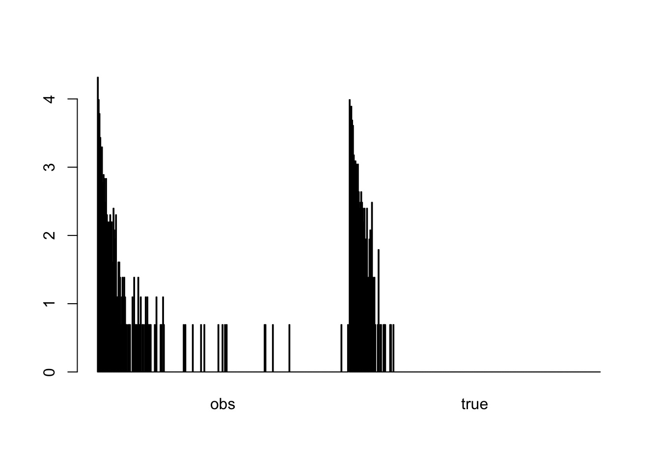
8.1.2 Fitting a non-hierarchical model leads to bias
normalModel = textConnection('
                             model {
                             # Priors
                             meanSize ~ dunif(1,100)

                             # Likelihood
                             for(i in 1:nObs){
                             true[i] ~ dexp(1/meanSize)
                             }
                             }
                             ')

# Bundle data
positiveObservations <- observations[observations>0]
data = list(true = positiveObservations, nObs=length(positiveObservations))

# Parameters to be monitored (= to estimate)
params = c("meanSize")

jagsModel = jags.model( file= normalModel , data=data, n.chains = 3, n.adapt= 500)
Compiling model graph
Resolving undeclared variables
Allocating nodes
Graph information:
Observed stochastic nodes: 500
Unobserved stochastic nodes: 1
Total graph size: 505
Initializing modelresults = coda.samples( jagsModel , variable.names=params,n.iter=5000)
plot(results)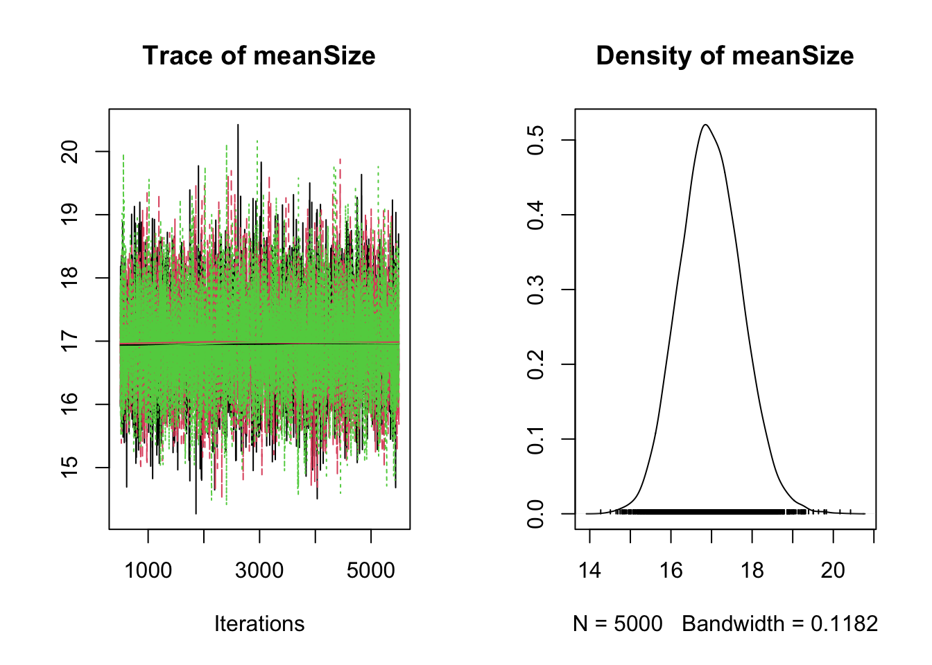
The main thing to note about this is that parameter estimates are heavily biased.
8.1.3 Fitting a hierarchical model removes the bias
Model specification if hierarchical model that accounts for the observation error in Jags
hierarchicalModel = textConnection('
model {
# Priors
meanSize ~ dunif(1,100)
sigma ~ dunif(0,20) # Precision 1/variance JAGS and BUGS use prec instead of sd
precision <- pow(sigma, -2)
# Likelihood
for(i in 1:nObs){
true[i] ~ dexp(1/meanSize)
observed[i] ~ dlnorm(log(true[i]), precision)
}
}
')
# Bundle data
data = list(observed = observations, nObs=length(observations))
# Parameters to be monitored (= to estimate)
params = c("meanSize", "sigma")
jagsModel = jags.model( file= hierarchicalModel , data=data, n.chains = 3, n.adapt= 500)Compiling model graph
Resolving undeclared variables
Allocating nodes
Graph information:
Observed stochastic nodes: 500
Unobserved stochastic nodes: 502
Total graph size: 1511
Initializing model#update(jagsModel, 2500) # updating without sampling
results = coda.samples( jagsModel , variable.names=params,n.iter=5000)
plot(results)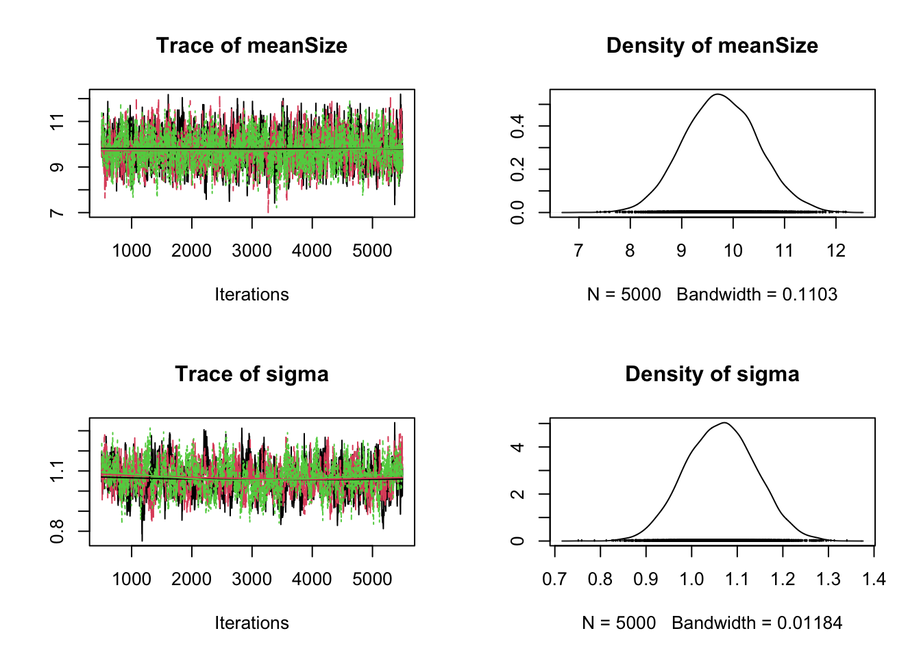
It’s always good to check the correlation structure in the posterior
8.2 Regression dilution in slope estimates
library(EcoData)
library(rjags)

nobs = nrow(volcanoisland)

# imagine we had a very bad measurement devide for the altitude
volcanoisland$sAltitudeR = volcanoisland$sAltitude + rnorm(nobs)

plot(log(windObs) ~ sAltitude, data = volcanoisland)
fit = lm(log(windObs) ~ sAltitude, data = volcanoisland)
summary(fit)
Call:
lm(formula = log(windObs) ~ sAltitude, data = volcanoisland)

Residuals:
    Min      1Q  Median      3Q     Max
-3.5295 -0.5738  0.0083  0.5897  2.3810

Coefficients:
            Estimate Std. Error t value Pr(>|t|)
(Intercept)  1.74308    0.02687   64.87   <2e-16 ***
sAltitude    0.41156    0.02688   15.31   <2e-16 ***
---
Signif. codes:  0 '***' 0.001 '**' 0.01 '*' 0.05 '.' 0.1 ' ' 1

Residual standard error: 0.8498 on 998 degrees of freedom
Multiple R-squared:  0.1902,    Adjusted R-squared:  0.1894
F-statistic: 234.3 on 1 and 998 DF, p-value: < 2.2e-16abline(fit, col = "red")
fit = lm(log(windObs) ~ sAltitudeR, data = volcanoisland)
summary(fit)
Call:
lm(formula = log(windObs) ~ sAltitudeR, data = volcanoisland)

Residuals:
    Min      1Q  Median      3Q     Max
-3.3499 -0.5476  0.0075  0.6033  2.5089

Coefficients:
            Estimate Std. Error t value Pr(>|t|)
(Intercept)  1.75802    0.02821   62.31   <2e-16 ***
sAltitudeR   0.21449    0.01938   11.07   <2e-16 ***
---
Signif. codes:  0 '***' 0.001 '**' 0.01 '*' 0.05 '.' 0.1 ' ' 1

Residual standard error: 0.8911 on 998 degrees of freedom
Multiple R-squared:  0.1094,    Adjusted R-squared:  0.1085
F-statistic: 122.5 on 1 and 998 DF, p-value: < 2.2e-16abline(fit, col = "blue")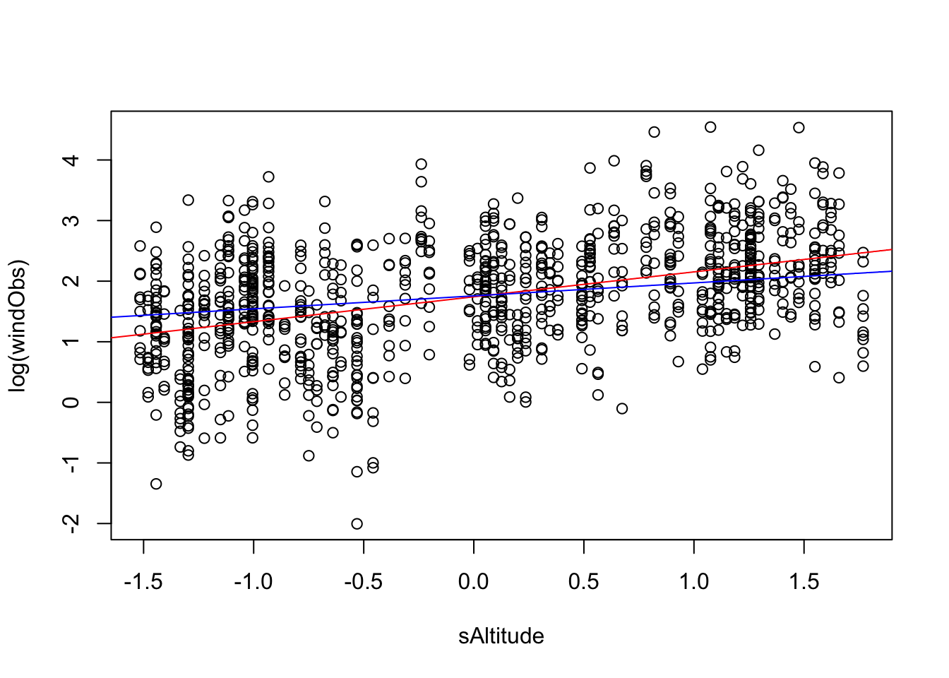
let’s see if we can correct the error
data = list(WindObs = log(volcanoisland$windObs),
            Altitude = volcanoisland$sAltitudeR,
            plot = as.numeric(volcanoisland$plot),
            nobs = nobs,
            nplots = length(unique(volcanoisland$plot)))


modelCode = "model{

  # Likelihood
  for(i in 1:nobs){

    # error on y
    WindObs[i] ~ dnorm(mu[i],tau)

    # error on x
    Altitude[i] ~ dnorm(TrueAltitude[plot[i]],tauMeasure)

    mu[i] <- AltitudeEffect*TrueAltitude[plot[i]]+ Intercept
  }

  # Prior distributions

  # For location parameters, normal choice is wide normal
  AltitudeEffect ~ dnorm(0,0.0001)
  Intercept ~ dnorm(0,0.0001)

  for(i in 1:nplots){
     TrueAltitude[i] ~ dnorm(0,0.0001)
  }

  # For scale parameters, normal choice is decaying
  tau ~ dgamma(0.001, 0.001)
  sigma <- 1/sqrt(tau)

  tauMeasure ~ dgamma(0.001, 0.001)
  sdMeasure <- 1/sqrt(tauMeasure)

}
"

jagsModel <- jags.model(file= textConnection(modelCode), data=data, n.chains = 3)
Compiling model graph
Resolving undeclared variables
Allocating nodes
Graph information:
Observed stochastic nodes: 2000
Unobserved stochastic nodes: 104
Total graph size: 3314
Initializing modelpara.names <- c("AltitudeEffect","Intercept","sigma", "sdMeasure")
Samples <- coda.samples(jagsModel, variable.names = para.names, n.iter = 5000)
plot(Samples)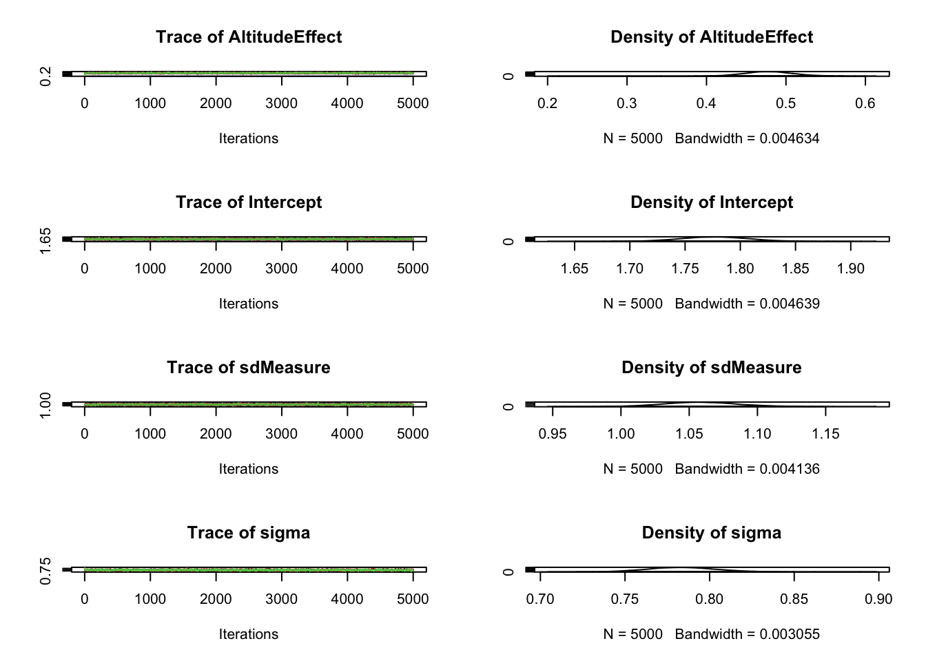
summary(Samples)
Iterations = 1:5000
Thinning interval = 1
Number of chains = 3
Sample size per chain = 5000

1. Empirical mean and standard deviation for each variable,
   plus standard error of the mean:

                 Mean      SD  Naive SE Time-series SE
AltitudeEffect 0.4789 0.03043 0.0002485      0.0004178
Intercept      1.7767 0.02995 0.0002445      0.0003376
sdMeasure      1.0588 0.02678 0.0002186      0.0002798
sigma          0.7837 0.01972 0.0001610      0.0002141

2. Quantiles for each variable:

                 2.5%    25%    50%    75%  97.5%
AltitudeEffect 0.4215 0.4585 0.4782 0.4986 0.5408
Intercept      1.7191 1.7565 1.7767 1.7970 1.8352
sdMeasure      1.0085 1.0405 1.0580 1.0763 1.1137
sigma          0.7463 0.7701 0.7833 0.7968 0.8233