10  State-space models

10.0.1 House marten example from Kery & Schaub

Based on the book “Bayesian population analysis using WinBUGS - a hierarchical perspective” by Marc K�ry & Michael Schaub (2012, Academic Press)

rm(list=ls())
library(R2jags)

model = "
model {
# Priors and constraints
logN[1] ~ dnorm(5.6, 0.01)       # Prior for initial population size
mean.r ~ dnorm(0, 0.001)             # Prior for mean growth rate
sigma.proc ~ dunif(0, 1)             # Prior for sd of state process
sigma2.proc <- pow(sigma.proc, 2)
tau.proc <- pow(sigma.proc, -2)
sigma.obs ~ dunif(0, 1)              # Prior for sd of observation process
sigma2.obs <- pow(sigma.obs, 2)
tau.obs <- pow(sigma.obs, -2)

# Likelihood
# State process
for (t in 1:(T-1)){
   r[t] ~ dnorm(mean.r, tau.proc)
   logN[t+1] <- logN[t] + r[t]
   }
# Observation process
for (t in 1:T) {
   y[t] ~ dnorm(logN[t], tau.obs)
   }

# Population sizes on real scale
for (t in 1:T) {
   N[t] <- exp(logN[t])
   }
}
"


# House martin population data from Magden
pyears <- 6 # Number of future years with predictions
hm.counts <- c(271, 261, 309, 318, 231, 216, 208, 226, 195, 226, 233, 209, 226, 192, 191, 225, 245, 205, 191, 174, rep(NA, pyears))
year <- 1990:(2009 + pyears)

# Bundle data
jags.data <- list(y = log(hm.counts), T = length(year))

# Initial values
inits <- function(){list(sigma.proc = runif(1, 0, 1), mean.r = rnorm(1), sigma.obs = runif(1, 0, 1), logN.est = c(rnorm(1, 5.6, 0.1), rep(NA, (length(year)-1))))}

# Parameters monitored
parameters <- c("r", "mean.r", "sigma2.obs", "sigma2.proc", "N")

# MCMC settings
ni <- 200000
nt <- 6
nb <- 100000
nc <- 3

# Call JAGS from R (BRT 3 min)
hm.ssm <- jags(jags.data, inits, parameters, textConnection(model), n.chains = nc, n.thin = nt, n.iter = ni, n.burnin = nb, working.directory = getwd())

module glm loaded

Compiling model graph
   Resolving undeclared variables
   Allocating nodes
Graph information:
   Observed stochastic nodes: 20
   Unobserved stochastic nodes: 35
   Total graph size: 118

Warning in jags.model(model.file, data = data, inits = init.values, n.chains =
n.chains, : Unused initial value for "logN.est" in chain 1

Warning in jags.model(model.file, data = data, inits = init.values, n.chains =
n.chains, : Unused initial value for "logN.est" in chain 2

Warning in jags.model(model.file, data = data, inits = init.values, n.chains =
n.chains, : Unused initial value for "logN.est" in chain 3

Initializing model

Summarize posteriors

print(hm.ssm, digits = 3)
plot(hm.ssm)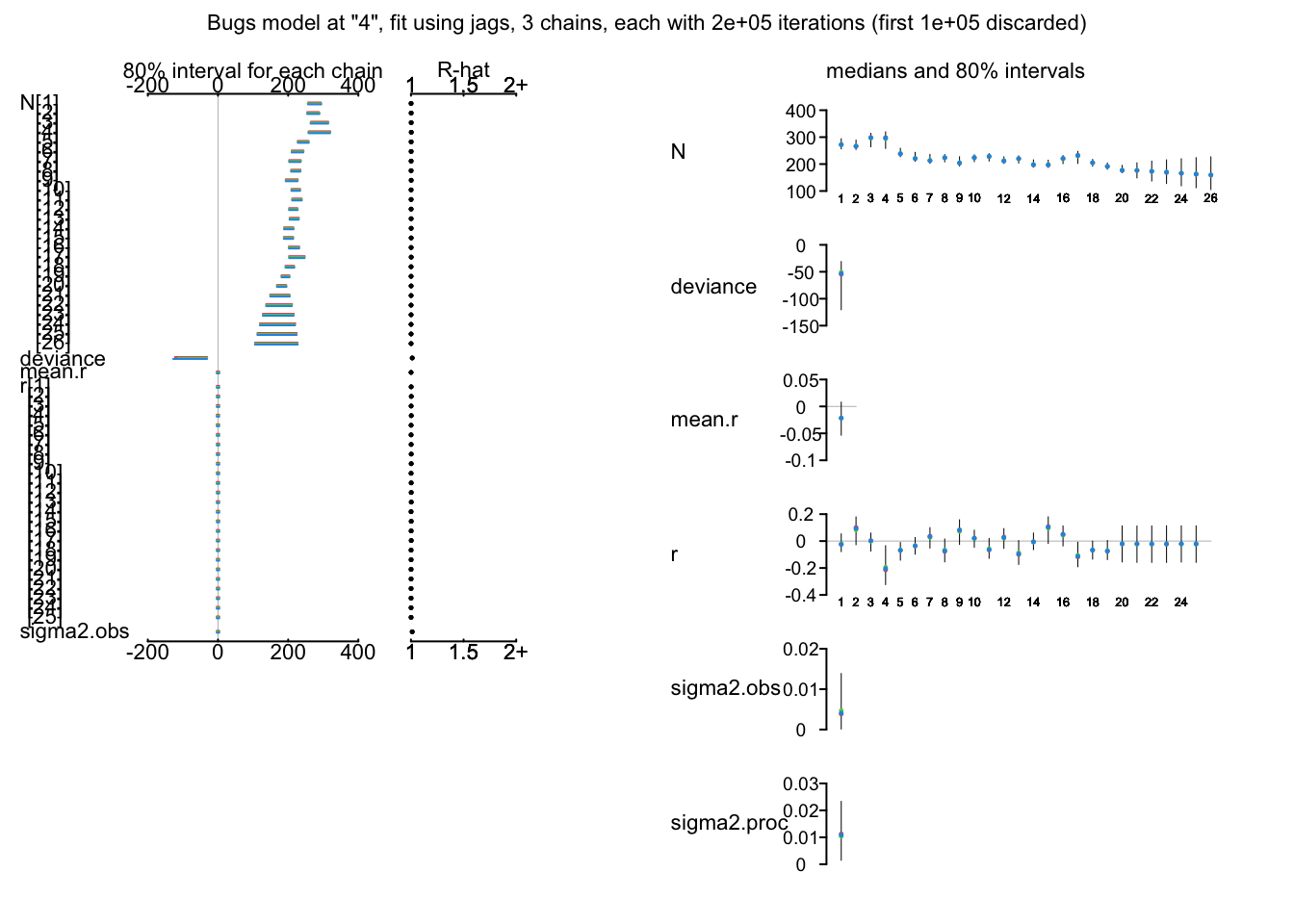

Draw figure

fitted <- lower <- upper <- numeric()
year <- 1990:2015
n.years <- length(hm.counts)
for (i in 1:n.years){
   fitted[i] <- mean(hm.ssm$BUGSoutput$sims.list$N[,i])
   lower[i] <- quantile(hm.ssm$BUGSoutput$sims.list$N[,i], 0.025)
   upper[i] <- quantile(hm.ssm$BUGSoutput$sims.list$N[,i], 0.975)}
m1 <- min(c(fitted, hm.counts, lower), na.rm = TRUE)
m2 <- max(c(fitted, hm.counts, upper), na.rm = TRUE)
par(mar = c(4.5, 4, 1, 1))
plot(0, 0, ylim = c(m1, m2), xlim = c(1, n.years), ylab = "Population size", xlab = "Year", col = "black", type = "l", lwd = 2, axes = FALSE, frame = FALSE)
axis(2, las = 1)
axis(1, at = 1:n.years, labels = year)
polygon(x = c(1:n.years, n.years:1), y = c(lower, upper[n.years:1]), col = "gray90", border = "gray90")
points(hm.counts, type = "l", col = "black", lwd = 2)
points(fitted, type = "l", col = "blue", lwd = 2)
legend(x = 1, y = 150, legend = c("Counts", "Estimates"), lty = c(1, 1), lwd = c(2, 2), col = c("black", "blue"), bty = "n", cex = 1)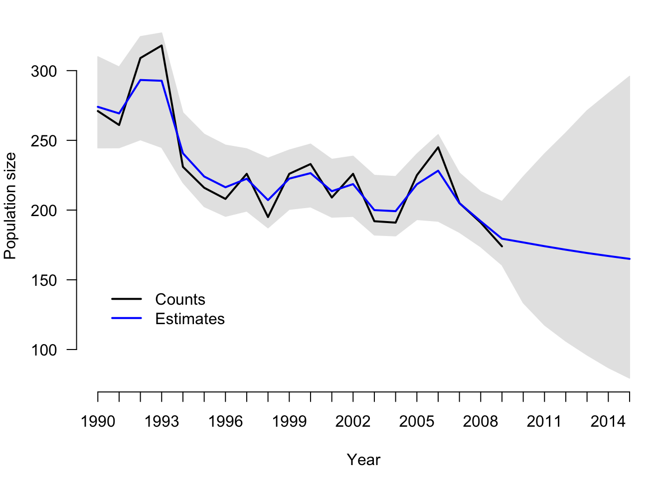

# Probability of N(2015) < N(2009)
mean(hm.ssm$BUGSoutput$sims.list$N[,26] < hm.ssm$BUGSoutput$mean$N[20])

[1] 0.6867875