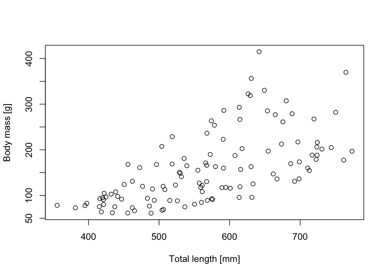
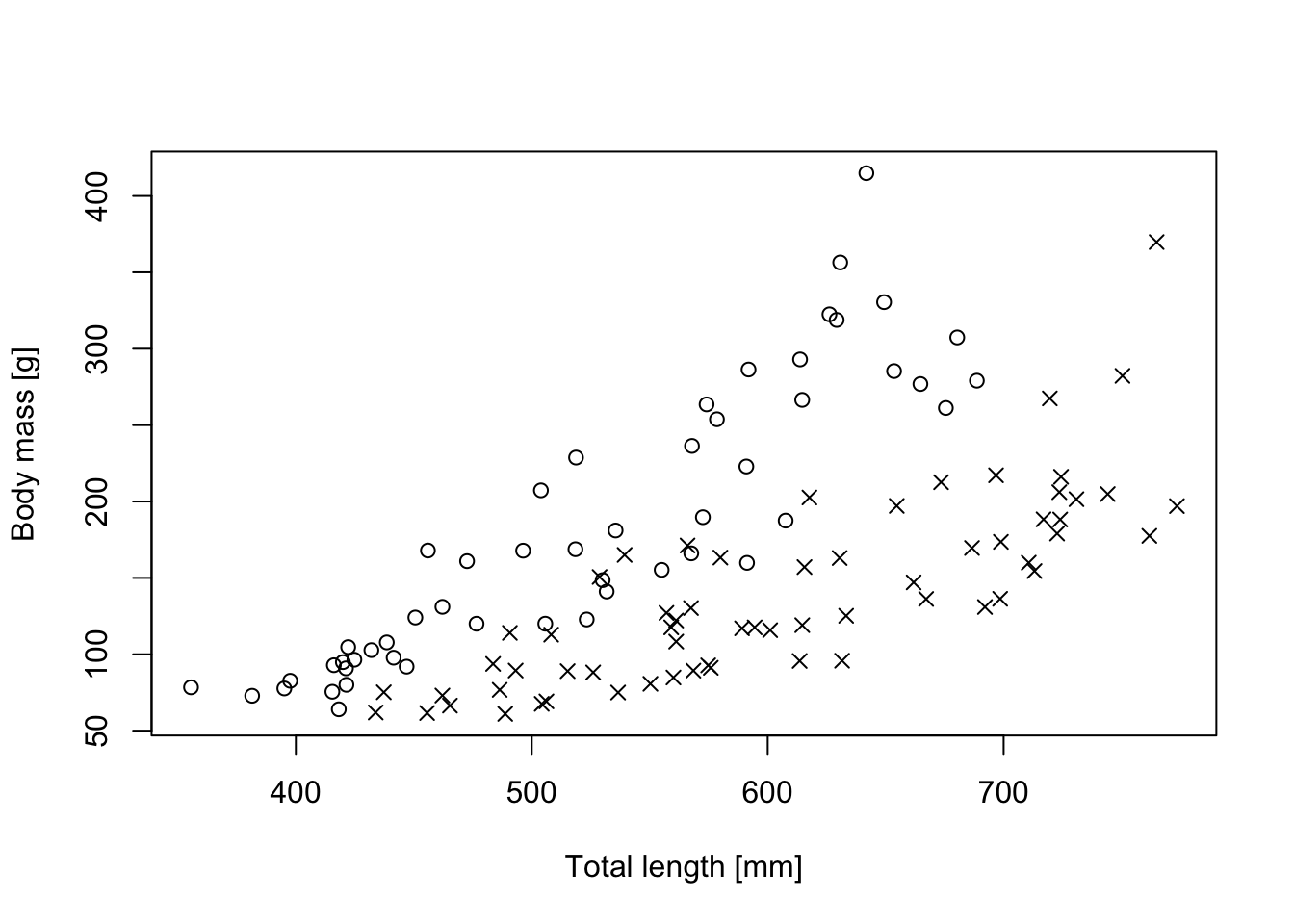
To introduce the typical options in a linear model, we use an example that was originally prepared by Jörn Pagel. In the example, we want to analyze predictors of Body mass in the snake Vipera aspis.
Dat =read.table("https://raw.githubusercontent.com/florianhartig/LearningBayes/master/data/Aspis_data.txt", stringsAsFactors = T)# Inspect relationship between body mass and total body lenghtplot(Dat$TL, Dat$BM,xlab ='Total length [mm]',ylab ='Body mass [g]')
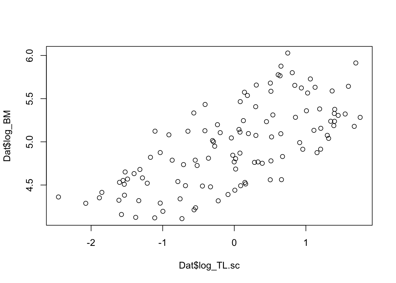
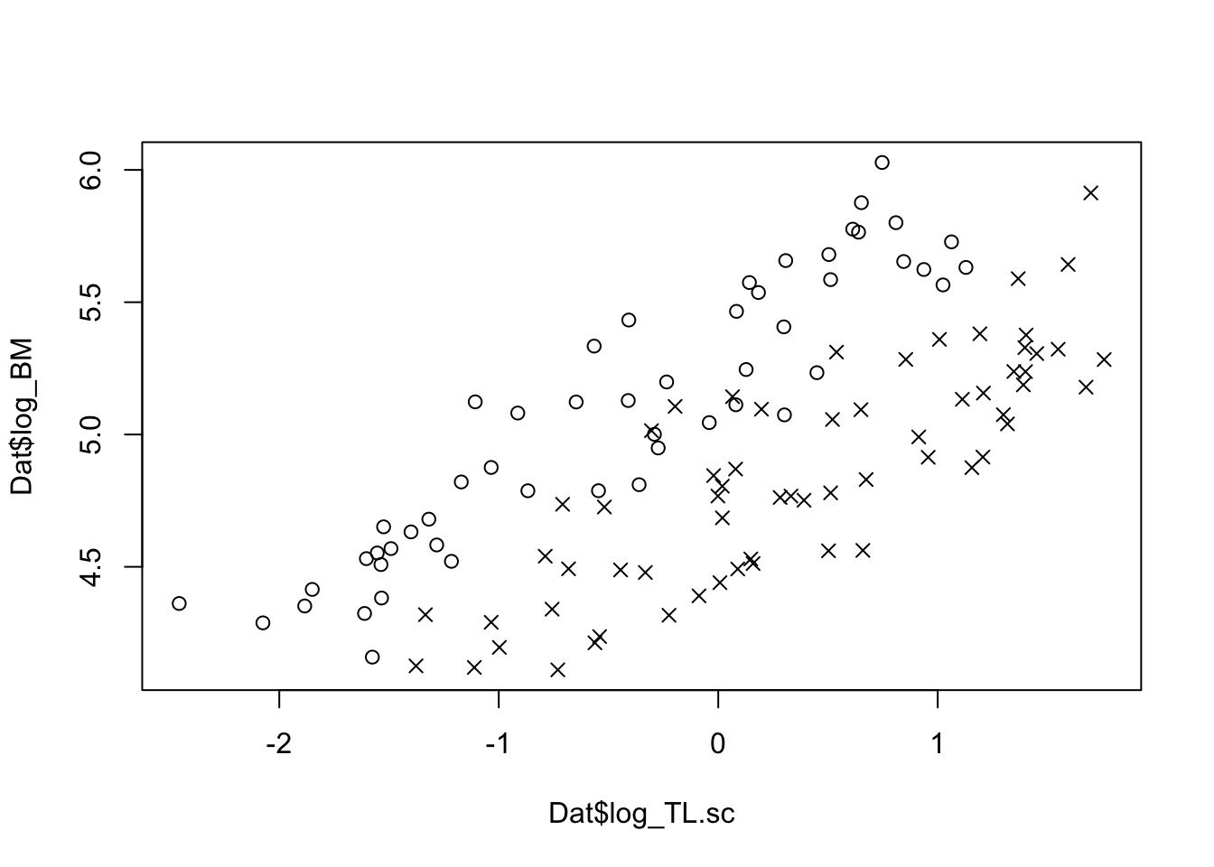
# For the analysis we use log-transformed body masses# and log-transformed and scaled total body lenght (TL)plot(Dat$log_TL.sc, Dat$log_BM)
4.1.1 LM with continous predictor
Linear regression with lm()
LM <-lm(log_BM ~ log_TL.sc, data = Dat)summary(LM)
Call:
lm(formula = log_BM ~ log_TL.sc, data = Dat)

Residuals:
     Min       1Q   Median       3Q      Max
-0.60635 -0.28199  0.01219  0.21303  0.83099

Coefficients:
            Estimate Std. Error t value Pr(>|t|)
(Intercept)  4.95347    0.03219  153.89   <2e-16 ***
log_TL.sc    0.32626    0.03233   10.09   <2e-16 ***
---
Signif. codes:  0 '***' 0.001 '**' 0.01 '*' 0.05 '.' 0.1 ' ' 1

Residual standard error: 0.3452 on 113 degrees of freedom
Multiple R-squared:  0.474, Adjusted R-squared:  0.4694
F-statistic: 101.8 on 1 and 113 DF,  p-value: < 2.2e-16
Analysis in JAGS
library(rjags)# 1) Save a description of the model in JAGS syntax # to the working directorymodel ="model{ # Likelihood for(i in 1:n.dat){ y[i] ~ dnorm(mu[i],tau) mu[i] <- alpha + beta.TL * TL[i] } # Prior distributions alpha ~ dnorm(0,0.001) beta.TL ~ dnorm(0,0.001) tau <- 1/(sigma*sigma) sigma ~ dunif(0,100) }"# s = function(x) dgamma(x, shape = 0.0001, rate = 0.001)# curve(s, 0, 5)# 2) Set up a list that contains all the necessary dataData =list(y = Dat$log_BM, TL = Dat$log_TL.sc,n.dat =nrow(Dat))# 3) Specify a function to generate inital values for the parametersinits.fn <-function() list(alpha =rnorm(1), beta.TL =rnorm(1),sigma =runif(1,1,100))# Compile the model and run the MCMC for an adaptation (burn-in) phasejagsModel <-jags.model(file =textConnection(model), data=Data, init = inits.fn, n.chains =3, n.adapt=5000)
Compiling model graph
   Resolving undeclared variables
   Allocating nodes
Graph information:
   Observed stochastic nodes: 115
   Unobserved stochastic nodes: 3
   Total graph size: 470

Initializing model
# Specify parameters for which posterior samples are savedpara.names <-c("alpha","beta.TL","sigma")# Continue the MCMC runs with samplingSamples <-coda.samples(jagsModel, variable.names = para.names, n.iter =5000)# Statistical summaries of the (marginal) posterior # distribution for each parametersummary(Samples)
Iterations = 5001:10000
Thinning interval = 1
Number of chains = 3
Sample size per chain = 5000

1. Empirical mean and standard deviation for each variable,
   plus standard error of the mean:

          Mean      SD  Naive SE Time-series SE
alpha   4.9532 0.03272 0.0002671      0.0002671
beta.TL 0.3259 0.03276 0.0002674      0.0002655
sigma   0.3491 0.02360 0.0001927      0.0002524

2. Quantiles for each variable:

          2.5%    25%    50%    75%  97.5%
alpha   4.8881 4.9310 4.9537 4.9751 5.0171
beta.TL 0.2619 0.3039 0.3259 0.3477 0.3905
sigma   0.3066 0.3327 0.3476 0.3639 0.3992
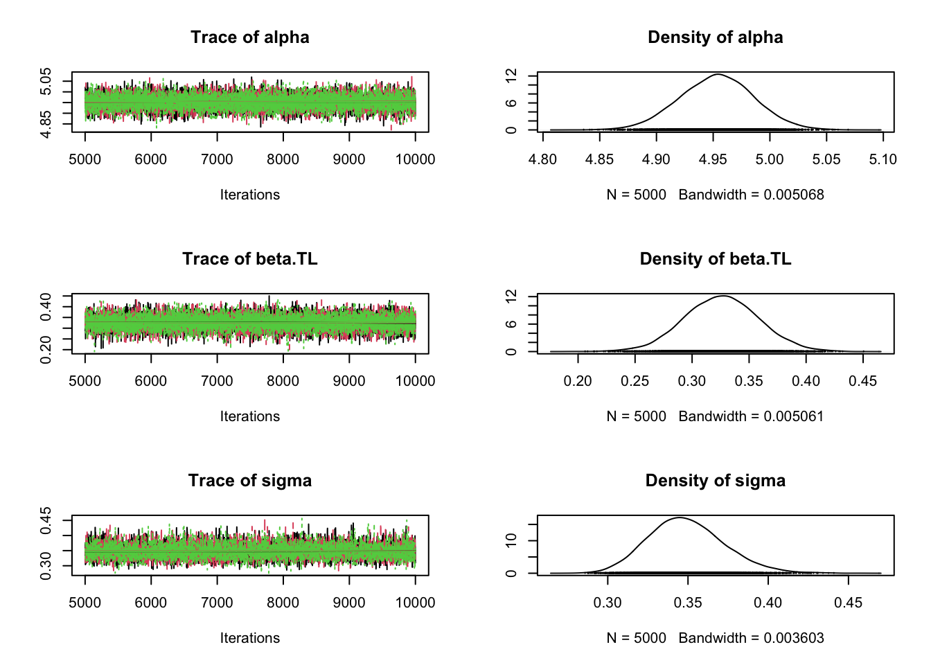
# If we were interested only in point estimates,# we could extract posterior meansPostMeans <-summary(Samples)$statistics[,'Mean']# Graphical overview of the samples from the MCMC chainsplot(Samples)
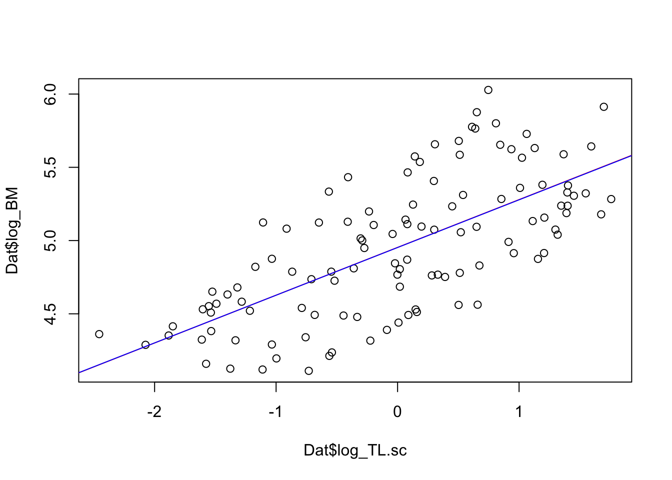
Compare this to the lm() results
plot(Dat$log_TL.sc, Dat$log_BM)coef(LM)
(Intercept)   log_TL.sc
  4.9534727   0.3262571
# and the two regression linesabline(LM, col ='red')abline(PostMeans[1:2], col ='blue')
4.1.2 LM with categorical predictor
Inspect relationship between body mass and total body lenght but now seperately for the two sexes
point.symbols <-c(f =1, m =4)plot(Dat$TL, Dat$BM,pch = point.symbols[Dat$Sex],xlab ='Total length [mm]',ylab ='Body mass [g]')
# For the analysis we use log-transformed body masses# and log-transformed and scaled total body lenght (TL)plot(Dat$log_TL.sc, Dat$log_BM, pch = point.symbols[Dat$Sex])
Linear regression with lm()
LM <-lm(log_BM ~ log_TL.sc + Sex, data = Dat)summary(LM)
Call:
lm(formula = log_BM ~ log_TL.sc + Sex, data = Dat)

Residuals:
     Min       1Q   Median       3Q      Max
-0.41822 -0.18030 -0.02969  0.16075  0.50885

Coefficients:
            Estimate Std. Error t value Pr(>|t|)
(Intercept)  5.27831    0.03127  168.81   <2e-16 ***
log_TL.sc    0.44765    0.02197   20.38   <2e-16 ***
Sexm        -0.59296    0.04394  -13.49   <2e-16 ***
---
Signif. codes:  0 '***' 0.001 '**' 0.01 '*' 0.05 '.' 0.1 ' ' 1

Residual standard error: 0.214 on 112 degrees of freedom
Multiple R-squared:  0.7997,    Adjusted R-squared:  0.7961
F-statistic: 223.6 on 2 and 112 DF,  p-value: < 2.2e-16
Analysis in JAGS
model ="model{ # Likelihood for(i in 1:n.dat){ y[i] ~ dnorm(mu[i],tau) mu[i] <- alpha + beta.TL * TL[i] + beta.m * Sexm[i] } # Prior distributions alpha ~ dnorm(0,0.001) beta.TL ~ dnorm(0,0.001) beta.m ~ dnorm(0,0.001) tau <- 1/(sigma*sigma) sigma ~ dunif(0,100) } "# 2) Set up a list that contains all the necessary dataData =list(y = Dat$log_BM, TL = Dat$log_TL.sc,Sexm =ifelse(Dat$Sex =='m', 1, 0),n.dat =nrow(Dat))# 3) Specify a function to generate inital values for the parametersinits.fn <-function() list(alpha =rnorm(1), beta.TL =rnorm(1),beta.m =rnorm(1),sigma =runif(1,1,100))# Compile the model and run the MCMC for an adaptation (burn-in) phasejagsModel <-jags.model(file =textConnection(model), data=Data, init = inits.fn, n.chains =3, n.adapt=5000)
Compiling model graph
   Resolving undeclared variables
   Allocating nodes
Graph information:
   Observed stochastic nodes: 115
   Unobserved stochastic nodes: 4
   Total graph size: 588

Initializing model
# Specify parameters for which posterior samples are savedpara.names <-c("alpha","beta.TL","beta.m","sigma")# Continue the MCMC runs with samplingSamples <-coda.samples(jagsModel, variable.names = para.names, n.iter =5000)# Statistical summaries of the (marginal) posterior distribution# for each parametersummary(Samples)
Iterations = 5001:10000
Thinning interval = 1
Number of chains = 3
Sample size per chain = 5000

1. Empirical mean and standard deviation for each variable,
   plus standard error of the mean:

           Mean      SD  Naive SE Time-series SE
alpha    5.2796 0.03207 0.0002619      0.0005402
beta.TL  0.4480 0.02231 0.0001821      0.0002520
beta.m  -0.5948 0.04525 0.0003694      0.0007766
sigma    0.2164 0.01467 0.0001198      0.0001537

2. Quantiles for each variable:

           2.5%     25%     50%     75%   97.5%
alpha    5.2165  5.2582  5.2793  5.3008  5.3439
beta.TL  0.4044  0.4330  0.4479  0.4631  0.4919
beta.m  -0.6847 -0.6246 -0.5946 -0.5647 -0.5065
sigma    0.1894  0.2061  0.2158  0.2258  0.2465
From the previous plot, it´s obvious that we could also consider an interaction between sex and body mass
Linear regression with lm()
LM <-lm(log_BM ~ log_TL.sc + Sex + Sex:log_TL.sc, data = Dat)summary(LM)
Call:
lm(formula = log_BM ~ log_TL.sc + Sex + Sex:log_TL.sc, data = Dat)

Residuals:
     Min       1Q   Median       3Q      Max
-0.40757 -0.16446 -0.01407  0.14330  0.51672

Coefficients:
               Estimate Std. Error t value Pr(>|t|)
(Intercept)     5.29416    0.03247 163.059   <2e-16 ***
log_TL.sc       0.48297    0.03049  15.841   <2e-16 ***
Sexm           -0.59513    0.04362 -13.642   <2e-16 ***
log_TL.sc:Sexm -0.07225    0.04361  -1.657      0.1
---
Signif. codes:  0 '***' 0.001 '**' 0.01 '*' 0.05 '.' 0.1 ' ' 1

Residual standard error: 0.2123 on 111 degrees of freedom
Multiple R-squared:  0.8045,    Adjusted R-squared:  0.7992
F-statistic: 152.3 on 3 and 111 DF,  p-value: < 2.2e-16
Analysis in JAGS
model ="model{ # Likelihood for(i in 1:n.dat){ y[i] ~ dnorm(mu[i],tau) mu[i] <- alpha + beta.TL[Sex[i]] * TL[i] + beta.m * Sexm[i] } # Prior distributions alpha ~ dnorm(0,0.001) for(s in 1:2){ beta.TL[s] ~ dnorm(0,0.001) } beta.m ~ dnorm(0,0.001) tau <- 1/(sigma*sigma) sigma ~ dunif(0,100) } "# 2) Set up a list that contains all the necessary dataData =list(y = Dat$log_BM, TL = Dat$log_TL.sc,Sexm =ifelse(Dat$Sex =='m', 1, 0),Sex =as.numeric(Dat$Sex),n.dat =nrow(Dat))# 3) Specify a function to generate inital values for the parametersinits.fn <-function() list(alpha =rnorm(1), beta.TL =rnorm(2),beta.m =rnorm(1),sigma =runif(1,1,100))# Compile the model and run the MCMC for an adaptation (burn-in) phasejagsModel <-jags.model(file =textConnection(model), data=Data, init = inits.fn, n.chains =3, n.adapt=5000)
Compiling model graph
   Resolving undeclared variables
   Allocating nodes
Graph information:
   Observed stochastic nodes: 115
   Unobserved stochastic nodes: 5
   Total graph size: 704

Initializing model
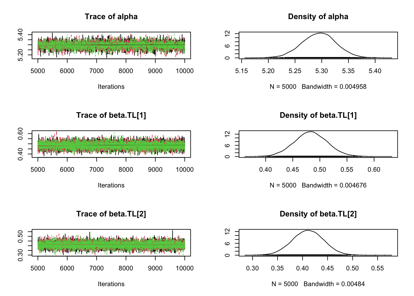
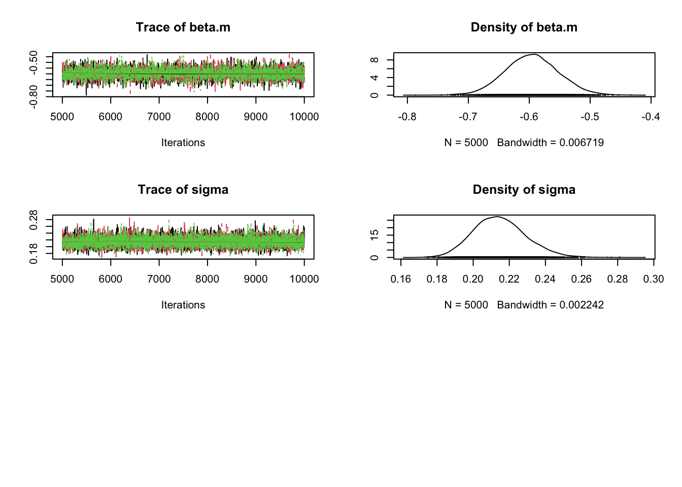
# Specify parameters for which posterior samples are savedpara.names <-c("alpha","beta.TL","beta.m","sigma")# Continue the MCMC runs with samplingSamples <-coda.samples(jagsModel, variable.names = para.names, n.iter =5000)# Statistical summaries of the (marginal) posterior distribution# for each parametersummary(Samples)
Iterations = 5001:10000
Thinning interval = 1
Number of chains = 3
Sample size per chain = 5000

1. Empirical mean and standard deviation for each variable,
   plus standard error of the mean:

              Mean      SD  Naive SE Time-series SE
alpha       5.2948 0.03231 0.0002638      0.0005270
beta.TL[1]  0.4833 0.03038 0.0002480      0.0003388
beta.TL[2]  0.4108 0.03124 0.0002551      0.0002972
beta.m     -0.5958 0.04369 0.0003567      0.0007299
sigma       0.2147 0.01465 0.0001196      0.0001593

2. Quantiles for each variable:

              2.5%     25%     50%     75%   97.5%
alpha       5.2316  5.2733  5.2953  5.3162  5.3577
beta.TL[1]  0.4238  0.4631  0.4831  0.5036  0.5436
beta.TL[2]  0.3496  0.3898  0.4109  0.4318  0.4717
beta.m     -0.6808 -0.6251 -0.5960 -0.5670 -0.5088
sigma       0.1884  0.2045  0.2139  0.2239  0.2456
##################################################################### Linear regression with lm()library(lme4)
Loading required package: Matrix
LME <-lmer(log_BM ~ log_TL.sc + Sex + Sex:log_TL.sc+ (1|Pop), data = Dat)summary(LME)
Linear mixed model fit by REML ['lmerMod']
Formula: log_BM ~ log_TL.sc + Sex + Sex:log_TL.sc + (1 | Pop)
   Data: Dat

REML criterion at convergence: -135.6

Scaled residuals:
     Min       1Q   Median       3Q      Max
-2.62996 -0.80341 -0.05736  0.71521  2.79946

Random effects:
 Groups   Name        Variance Std.Dev.
 Pop      (Intercept) 0.03569  0.1889
 Residual             0.01152  0.1073
Number of obs: 115, groups:  Pop, 9

Fixed effects:
               Estimate Std. Error t value
(Intercept)     5.30770    0.06515  81.468
log_TL.sc       0.50259    0.01676  29.996
Sexm           -0.59752    0.02243 -26.643
log_TL.sc:Sexm -0.04369    0.02291  -1.907

Correlation of Fixed Effects:
            (Intr) lg_TL. Sexm
log_TL.sc    0.102
Sexm        -0.191 -0.297
lg_TL.sc:Sx -0.071 -0.656  0.016
############################################################## Analysis in JAGS ##############################################################model ="model{ # Likelihood for(i in 1:n.dat){ y[i] ~ dnorm(mu[i],tau) mu[i] <- alpha[Pop[i]] + beta.TL[Sex[i]] * TL[i] + beta.m * Sexm[i] } # Prior distributions for(p in 1:n.pop){ alpha[p] ~ dnorm(mu.alpha, tau.pop) } for(s in 1:2){ beta.TL[s] ~ dnorm(0,0.001) } mu.alpha ~ dnorm(0,0.001) beta.m ~ dnorm(0,0.001) tau <- 1/(sigma*sigma) sigma ~ dunif(0,100) tau.pop <- 1/(sigma.pop*sigma.pop) sigma.pop ~ dunif(0,100) } "# 2) Set up a list that contains all the necessary dataData =list(y = Dat$log_BM, TL = Dat$log_TL.sc,Sexm =ifelse(Dat$Sex =='m', 1, 0),Sex =as.numeric(Dat$Sex),n.dat =nrow(Dat),Pop = Dat$Pop,n.pop =max(Dat$Pop))# 3) Specify a function to generate inital values for the parametersinits.fn <-function() list(mu.alpha =rnorm(1), beta.TL =rnorm(2),beta.m =rnorm(1),sigma =runif(1,1,100),sigma.pop =runif(1,1,100))# Compile the model and run the MCMC for an adaptation (burn-in) phasejagsModel <-jags.model(file =textConnection(model), data=Data, init = inits.fn, n.chains =3, n.adapt=5000)
Compiling model graph
   Resolving undeclared variables
   Allocating nodes
Graph information:
   Observed stochastic nodes: 115
   Unobserved stochastic nodes: 15
   Total graph size: 832

Initializing model
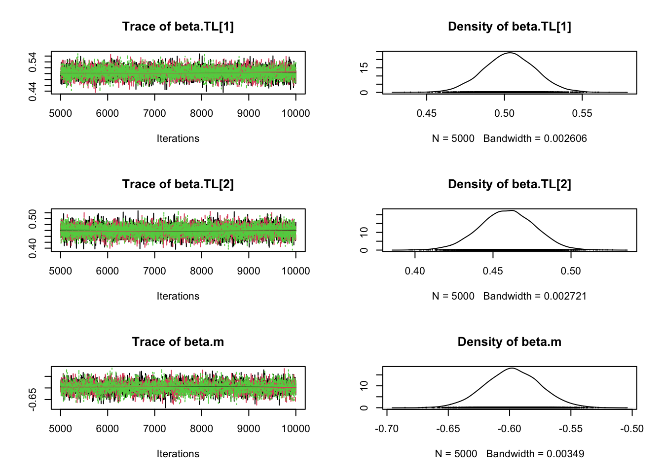
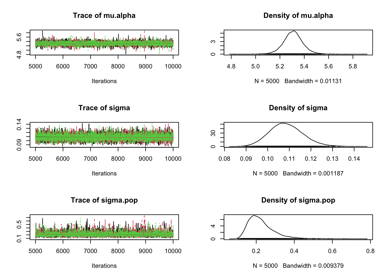
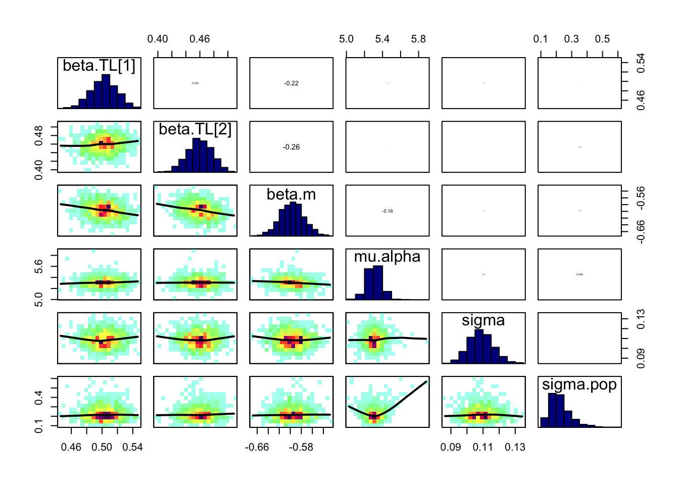
# Specify parameters for which posterior samples are savedpara.names <-c("mu.alpha","beta.TL","beta.m","sigma","sigma.pop")# Continue the MCMC runs with samplingSamples <-coda.samples(jagsModel, variable.names = para.names, n.iter =5000)# Statistical summaries of the (marginal) posterior distribution# for each parametersummary(Samples)
Iterations = 5001:10000
Thinning interval = 1
Number of chains = 3
Sample size per chain = 5000

1. Empirical mean and standard deviation for each variable,
   plus standard error of the mean:

              Mean       SD  Naive SE Time-series SE
beta.TL[1]  0.5032 0.016849 0.0001376      2.026e-04
beta.TL[2]  0.4590 0.017565 0.0001434      1.980e-04
beta.m     -0.5974 0.022529 0.0001839      3.829e-04
mu.alpha    5.3083 0.080623 0.0006583      7.273e-04
sigma       0.1087 0.007728 0.0000631      8.905e-05
sigma.pop   0.2261 0.070652 0.0005769      1.074e-03

2. Quantiles for each variable:

               2.5%     25%     50%     75%   97.5%
beta.TL[1]  0.47004  0.4920  0.5032  0.5145  0.5362
beta.TL[2]  0.42407  0.4474  0.4591  0.4709  0.4930
beta.m     -0.64159 -0.6125 -0.5975 -0.5822 -0.5528
mu.alpha    5.14824  5.2592  5.3084  5.3570  5.4702
sigma       0.09469  0.1033  0.1082  0.1136  0.1251
sigma.pop   0.13155  0.1773  0.2126  0.2585  0.4013
# Compare this to the lmer() resultssummary(LME)
Linear mixed model fit by REML ['lmerMod']
Formula: log_BM ~ log_TL.sc + Sex + Sex:log_TL.sc + (1 | Pop)
   Data: Dat

REML criterion at convergence: -135.6

Scaled residuals:
     Min       1Q   Median       3Q      Max
-2.62996 -0.80341 -0.05736  0.71521  2.79946

Random effects:
 Groups   Name        Variance Std.Dev.
 Pop      (Intercept) 0.03569  0.1889
 Residual             0.01152  0.1073
Number of obs: 115, groups:  Pop, 9

Fixed effects:
               Estimate Std. Error t value
(Intercept)     5.30770    0.06515  81.468
log_TL.sc       0.50259    0.01676  29.996
Sexm           -0.59752    0.02243 -26.643
log_TL.sc:Sexm -0.04369    0.02291  -1.907

Correlation of Fixed Effects:
            (Intr) lg_TL. Sexm
log_TL.sc    0.102
Sexm        -0.191 -0.297
lg_TL.sc:Sx -0.071 -0.656  0.016
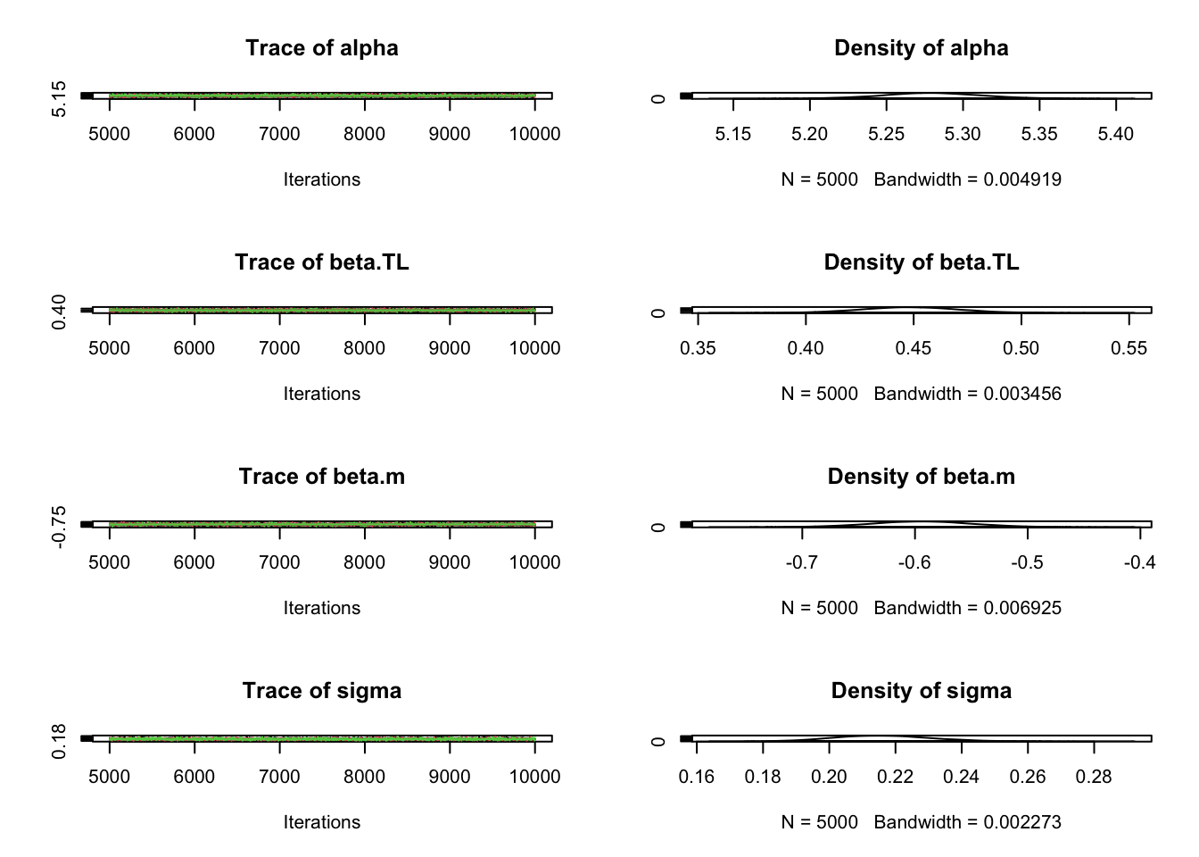
# Graphical overview of the samples from the MCMC chainsplot(Samples)