Standard GOF metrics Startvalues for sampling with nrChains > 1 : if you want to provide different start values for the different chains, provide a list
Standard GOF metrics Startvalues for sampling with nrChains > 1 : if you want to provide different start values for the different chains, provide a list
GOF(observed, predicted, plot = F)
Arguments
| observed | observed values |
|---|---|
| predicted | predicted values |
| plot | should a plot be created |
Value
A list with the following entries: rmse = root mean squared error, mae = mean absolute error, slope = slope of regression, offset = intercept of regression, R2 = R2 of regression
Details
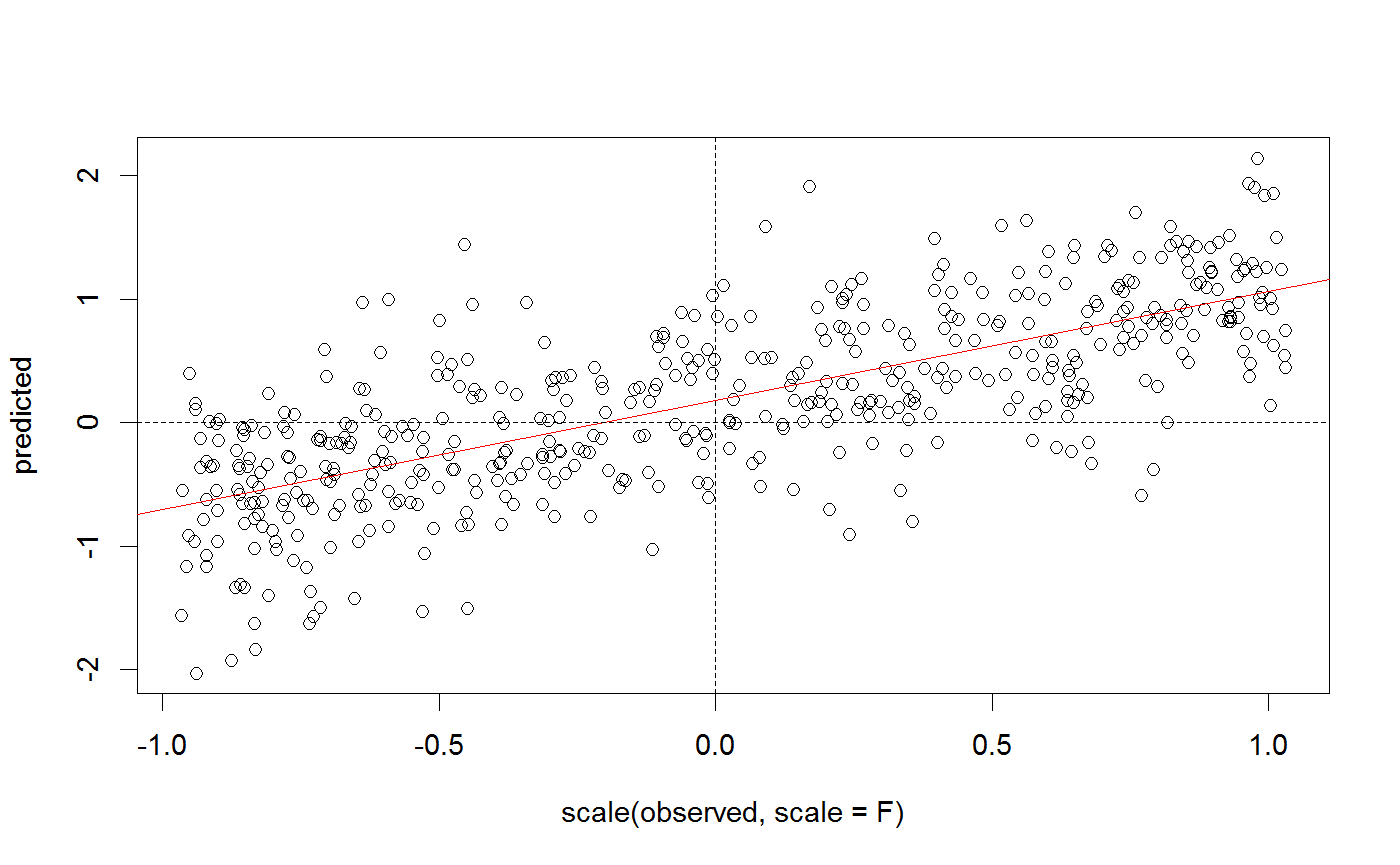
The function considers predicted ~ observed and calculates
1) rmse = root mean squared error 2) mae = mean absolute errorr 3) a linear regression with slope, intercept and coefficient of determination R2
For the linear regression, the x axis is centered, meaning that the intercept is the difference between observed / predicted for the MEAN predicted value. This setting avoids a correlation between slope and intercept (that the intercept is != 0 as soon as the slope is !=0)
Examples
x = runif(500,-1,1) y = 0.2 + 0.9 *x + rnorm(500, sd = 0.5) summary(lm(y ~ x))#> #> Call: #> lm(formula = y ~ x) #> #> Residuals: #> Min 1Q Median 3Q Max #> -1.44986 -0.30138 -0.02512 0.33049 1.66535 #> #> Coefficients: #> Estimate Std. Error t value Pr(>|t|) #> (Intercept) 0.20840 0.02258 9.23 <2e-16 *** #> x 0.88446 0.03645 24.27 <2e-16 *** #> --- #> Signif. codes: 0 ‘***’ 0.001 ‘**’ 0.01 ‘*’ 0.05 ‘.’ 0.1 ‘ ’ 1 #> #> Residual standard error: 0.5041 on 498 degrees of freedom #> Multiple R-squared: 0.5418, Adjusted R-squared: 0.5409 #> F-statistic: 588.9 on 1 and 498 DF, p-value: < 2.2e-16 #>GOF(x,y)#> $rmse #> [1] 0.5506948 #> #> $mae #> [1] 0.4308861 #> #> $slope #> [1] 0.8844614 #> #> $offset #> [1] 0.17963 #> #> $R2 #> [1] 0.5418068 #>GOF(x,y, plot = TRUE)#> $rmse #> [1] 0.5506948 #> #> $mae #> [1] 0.4308861 #> #> $slope #> [1] 0.8844614 #> #> $offset #> [1] 0.17963 #> #> $R2 #> [1] 0.5418068 #>
